How to use these slides
<space>: go to the next slide<shift+space>: go back<left right up down arrows>: navigate through the presentation structure<esc>: toggle overview mode

These lecture notes and exercises are licensed under a Creative Commons Attribution 4.0 International License (CC BY 4.0)
Organizational
Exam
What? Will be an oral exam: 30 min preparation, 30 min questions.
When? first week or last week of February. Choose your examination time slot on our google sheet (first come, first serve).
How will the exam look like?
- we meet in my office
- topic + list of questions assigned randomly at arrival
- 30 minutes preparation: I will provide a computer (linux with internet)
- 30 minutes questions
What will be tested for?
- ability to read and understand code from freely available scientific software
- ability to explain a code structure / algorithm
- knowledge of the core concepts and semantics learned during the lecture
- ability to solve a programming problem and plan a programming task
If you worked regularly during the semester and learned the bold elements in the lecture notes you should be good to go!
Program for the last weeks
- Today: scientific python
- Next week: last lecture on open source + project time (+ would you like to present your climvis work???)
- Last week: pelita tournament (deadline for player submission at 8pm the day before)
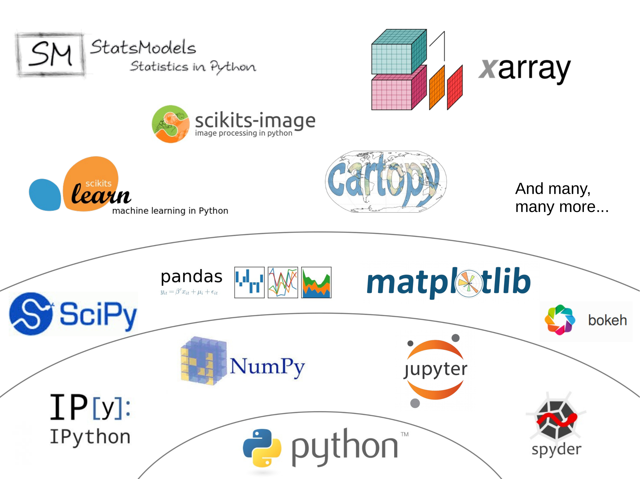
The scientific python stack
Pandas: fast, flexible, and expressive data structures
import pandas as pd
import io
import requests
import matplotlib.pyplot as plt
%matplotlib inline

url = ('https://stats.oecd.org/sdmx-json/data/DP_LIVE/.MEATCONSUMP.../OECD?'
       'contentType=csv&detail=code&separator=comma&csv-lang=en')
s = requests.get(url).content
df = pd.read_csv(io.StringIO(s.decode('utf-8')))
The power of split-apply-combine
df.loc[(df.LOCATION == 'USA') & (df.MEASURE=='KG_CAP')].groupby('TIME').sum().Value.plot(label='USA');
df.loc[(df.LOCATION == 'EU27') & (df.MEASURE=='KG_CAP')].groupby('TIME').sum().Value.plot(label='EU27');
df.loc[(df.LOCATION == 'CHN') & (df.MEASURE=='KG_CAP')].groupby('TIME').sum().Value.plot(label='CHN');
df.loc[(df.LOCATION == 'IND') & (df.MEASURE=='KG_CAP')].groupby('TIME').sum().Value.plot(label='IND');
plt.legend();

groups = df.loc[(df.LOCATION == 'USA') & (df.MEASURE=='KG_CAP')].groupby(['SUBJECT', 'TIME'])
groups['Value'].sum().unstack(level=0).plot();

xarray: pandas for N-dimensional data

numpy.array
import numpy as np
a = np.array([[1, 3, 9], [2, 8, 4]])
a
a[1, 2]
a.mean(axis=0)
xarray.DataArray
import xarray as xr
da = xr.DataArray(a, dims=['lat', 'lon'],
                  coords={'lon':[11, 12, 13], 'lat':[1, 2]})
da
da.sel(lon=13, lat=2)
da.mean(dim='lat')
Arithmetics
Broadcasting

a = xr.DataArray(np.arange(3), dims='time',
                 coords={'time':np.arange(3)})
b = xr.DataArray(np.arange(4), dims='space',
                 coords={'space':np.arange(4)})
a + b
Alignment

a = xr.DataArray(np.arange(3), dims='time',
                 coords={'time':np.arange(3)})
b = xr.DataArray(np.arange(5), dims='time',
                 coords={'time':np.arange(5)+1})
a + b
(Big) data: multiple files
Opening all files in a directory...
mfs = '/home/mowglie/disk/Data/Gridded/GPM/3BDAY_sorted/*.nc'
dsmf = xr.open_mfdataset(mfs, combine='by_coords')
... results in a consolidated dataset ...
dsmf
... on which all usual operations can be applied:
dsmf = dsmf.sel(time='2015')
dsmf
Yes, even computations!
ts = dsmf.precipitationCal.mean(dim=['lon', 'lat'])
ts
Computations are done "lazily"
No actual computation has happened yet:
ts.data
But they can be triggered:
ts = ts.load()
ts
ts.plot();
ts.rolling(time=31, center=True).mean().plot();

Have fun with Python in your studies and beyond!
... when will you have to use programming again in your master? I asked your teachers:
- Cryosphere in the Climate system: surface energy balance (pandas and Jupyter notebooks)
- Field Course in Atmospheric Sciences: analyze your field data (use whatever language you want)
- Mountain Meteorology: visualization of mountain wave solutions (open / Matlab)
- GFD (open)
- Radiation and remote sensing (open / Matlab)
- Atmospheric Chemistry and Remote sensing (Matlab)
- Master thesis (most of you will choose Python)
- ... and probably more!