Assignment #06: small exercises for Big Science
Exercise #06-01: indexing
Given a 2D numpy array defined as:
In [1]:
import numpy as np
x = np.array([[1, 2, 3],
              [4, 5, 6]])
The following indexing operations all select the same values out of the array:
x[:, 1]x[slice(0, 2, 1), 1]x[(slice(0, 2, 1), 1)]x[slice(0, 2, 1), slice(1, 2, 1)]x[..., 1]x[::1, 1]x[[0, 1], 1]x[:, -2]x[:, 1:2]x[:, [1]]
This can be checked with the following test:
In [2]:
from numpy.testing import assert_equal

ref = 7

assert_equal(ref, x[:, 1].sum())
assert_equal(ref, x[..., 1].sum())
assert_equal(ref, x[::1, 1].sum())
assert_equal(ref, x[slice(0, 2, 1), 1].sum())
assert_equal(ref, x[(slice(0, 2, 1), 1)].sum())
assert_equal(ref, x[slice(0, 2, 1), slice(1, 2, 1)].sum())
assert_equal(ref, x[[0, 1], 1].sum())
assert_equal(ref, x[:, -2].sum())
assert_equal(ref, x[:, 1:2].sum())
assert_equal(ref, x[:, [1]].sum())
Questions:
- What is the
...syntax doing? Again, it is the literal equivalent of an actual python object: what is it? - some of these indexing operations are truly equivalent to the "obvious" one,
x[:, 1]. List them. - Classify these operations (i) in basic and advanced operations, and (ii) by the shape of their output. Explain.
- I'd like my array
a = x[:, 1:2]to have a shape of (2, ) like most of the other operations listed above. What can I do to reshape it?
Exercise #06-02: the difference
Consider the following example:
In [3]:
a = np.array([1, 2, 3])
b = a
c = a

b = a - 10
c -= 100
What will be the values printed by print(a, b, c) after this code snippet? Explain.
Exercise #06-03: Greenwich
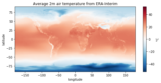
ERA-Interim reanalysis provides global atmospheric fields from 1979 to today. Someone prepared a grid of average temperature available here:
In [4]:
from urllib.request import Request, urlopen
from io import BytesIO
import json

# Parse the given url
url = 'https://github.com/fmaussion/scientific_programming/raw/master/data/monthly_temp.npz'
req = urlopen(Request(url)).read()
with np.load(BytesIO(req)) as data:
    temp = data['temp']
    lon = data['lon']
    lat = data['lat']
However, the data is not well processed! The longitudes are ranging from 0 to 360°, thus cutting UK and Africa in half! Reorganize the data and the corresponding coordinate to obtain a plot similar to this one:

Back to the table of contents