Assignments

Week 04

“Due date”: 24.04.2023

Exercise 01: a short programming riddle

Let’s read some output of the OGGM model (download the data):

import xarray as xr
with xr.open_dataset('../data/oggm_fl_ela.nc') as ds:
    ds = ds.load()

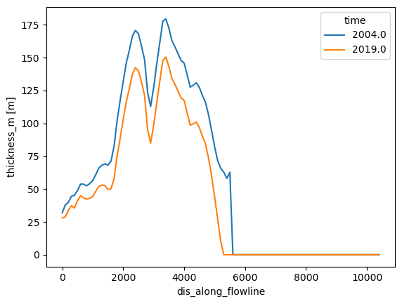
ds.thickness_m.sel(time=[2004, 2019]).plot(hue='time');

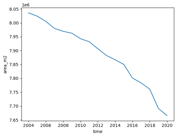
ds.area_m2.sum(dim='dis_along_flowline').plot();

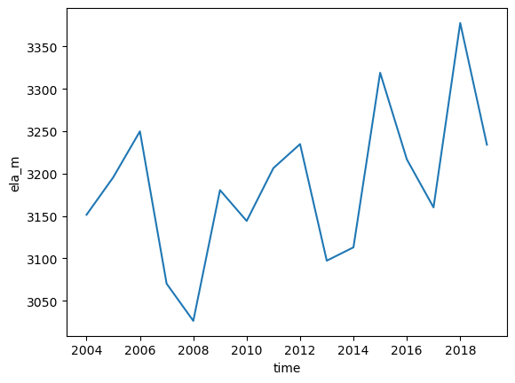
ds.ela_m.plot();

These data represent a glacier simulation using the flowline representation. Each grid point on the flowline has a width, an area, and a thickness changing with time:

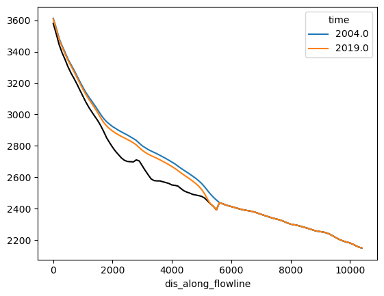
ds.bed_h.plot(color='k');

surface_h = ds.bed_h + ds.thickness_m
surface_h.sel(time=[2004, 2019]).plot(hue='time');

Your task is to compute the yearly “accumulation area ratio” (AAR), which is a number between 0 and 1 representing the fraction of the glacier area which is above the equilibrium line altitude (ELA). You have all the data you need above:

• ds.ela_m represents the equilibrium line altitude (ELA) each year (unit: m)

• surface_h represents the surface elevation of the glacier grid points each year (unit: m). With this you can check which grid points are located above the ELA.

• ds.area_m2 represents the area of each grid point each year (same dimensions as surface_h, unit: m2). With this you can compute the total area of the glacier each year (plotted above) and together with the ELA and surface_h you can compute the AAR.

The “difficulty” of this programming exercise is that all variables change each year. An intuitive way to solve the problem would be to use a for loop and you may want to start with this if you want to.

In fact, one can do it without for loop in 4 lines of code in xarray or numpy (the code in xarray is simpler than in pure numpy). If the task using xarray was too easy for you, you can try to code without xarray.

Exercise 02: code profiling

Pydemic is an agent-based model of a pandemic used to teach OOP to master students.

The code is very slow, because it does not use vectors to represent data. Each agent in the model has a location and state stored in scalar variables. This is OK given the purpose of the tool (teaching OOP), but we can still do better.

Run the pydemic.py module (no installation needed, a python pydemic.py should suffice to create a plot) and spend some time studying its code (it should be relatively straightforward). The code is quite slow though (a single simulation takes about 23s on my laptop).

Your task is to profile pydemic and find at least one bottleneck in the code. For the profiling, use the python profiler (maybe with snakeviz) or py-spy and run the module (remove the plot function from __main__ first!!!). Once you have found the bottleneck, you may implement or design a strategy to address it (implementation is optional).

Week 05: Numerical modelling

“Due date”: 08.05.2022

The glacier_model.py script (shift + right click to download) contains numerical code to realize glacier flowline experiments. The code is similar to what OGGM is doing, but with some simplifications:

• the glacier has a rectangular bed shape and is of constant width

• the mass balance is a simple linear function of elevation

The model solves the continuity equation as a numerical diffusion problem (see the seminal paper by Oerlemans 1997 if you are interested about the origins of such models: our code is the same but without the trapezoid shape and without basal sliding). There are a few things to say about the time stepping scheme (which is fixed to a constant value which is a bad idea), but numerics are not what we are trying to improve here.

Let’s consider the following:

from glacier_model import glacier_evolution
import matplotlib.pyplot as plt
import numpy as np
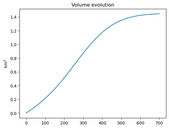
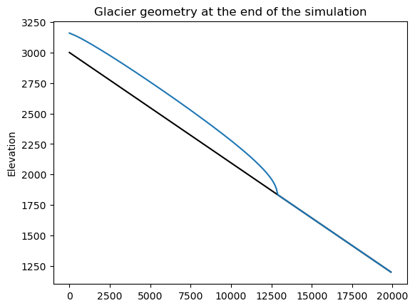
xc, bed_h, surface_h, years, volume, length = glacier_evolution()

plt.plot(years, volume*1e-9); plt.title('Volume evolution'); plt.ylabel('km$^{3}$');

plt.plot(xc, bed_h, color='k'); plt.plot(xc, surface_h);
plt.title('Glacier geometry at the end of the simulation'); plt.ylabel('Elevation');

%timeit glacier_evolution()

1.75 s ± 20.9 ms per loop (mean ± std. dev. of 7 runs, 1 loop each)

Let’s make this code faster in two steps (which is also what you should do in real life)

“Micro-“optimizations

Your task: profile the code and evaluate the bottlenecks, and optimize what can be optimized.

With a few very simple changes in the code (all related to the examples discussed in the lecture notes), I was able to make the code faster by a factor of two:

from glacier_model_optim import glacier_evolution_optim
%timeit glacier_evolution_optim()

Im at the top level

1.5 s ± 11.8 ms per loop (mean ± std. dev. of 7 runs, 1 loop each)

Multiprocessing

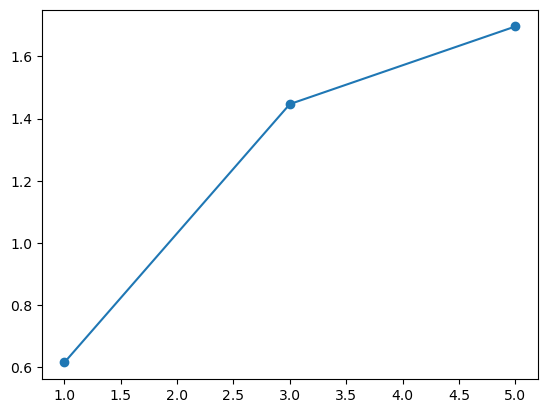
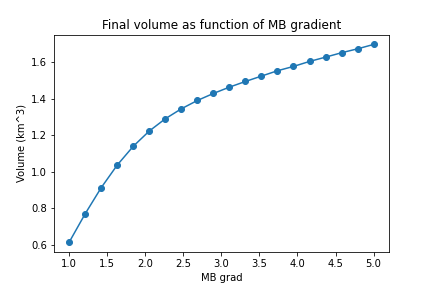
Let’s consider the following sensitivity experiments (taking way too long):

volumes = []
grads = np.linspace(1, 5, 3)
for grad in grads:
    xc, bed_h, surface_h, years, volume, length = glacier_evolution_optim(mb_grad=grad)
    volumes.append(volume)
volumes = np.array(volumes)

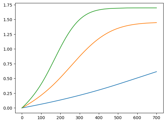
plt.plot(grads, volumes[:, -1] * 1e-9, 'o-');

plt.plot(years, volumes.T * 1e-9);

What if we want to make 100 experiments instead of 3?

The problem is what we call embarrassingly parallel: each task is fully independent of the others.

Use python’s multiprocessing Pool.map() method to realize the same experiments on the MB gradient but with input np.linspace(1, 5, 20) instead.

The output plot should look more something like:

Repeat with another sensitivity experiment of your choice!