Lambert conformal projection

High-latitude areas should rather be plotted on an area-conserving projection. In the few lines of code below you find some examples to get you started.

First, the imports. They are the same as always, but I removed the figure size defaults:

# Import the tools we are going to need today:
import matplotlib.pyplot as plt  # plotting library
import numpy as np  # numerical library
import xarray as xr  # netCDF library
import cartopy  # Map projections libary
import cartopy.crs as ccrs  # Projections list

Read and select the regional data

Reading the data works as always:

ds = xr.open_dataset('../data/ERA5_LowRes_Invariant.nc')

To select the data for a specific region, we will use xray’s sel function as we learned in the exercises. I’ve made a pre-selection for you but you are free to make the domain bigger/smaller if you find it useful for your analyses! Just uncomment the two lines relevant for your case:

# North-America -- note that I have to make the domain much larger in order to "fill" the plot below
ds = ds.sel(latitude=slice(80, 10), longitude=slice(-180, 0))
plt.rcParams['figure.figsize'] = (10, 6)

Note that I set the standard figure size for each region. You can always change those, and also make plots of any size later on (examples below).

Now we read the variable:

z = ds.z / 9.81

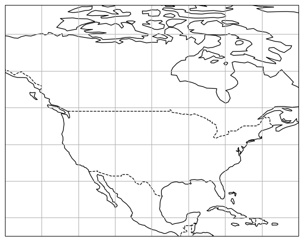
Define the projection

ax = plt.axes(projection=ccrs.PlateCarree())
ax.set_extent([-140, -60, 15, 75], ccrs.Geodetic())
ax.coastlines(); ax.gridlines();
ax.add_feature(cartopy.feature.BORDERS, linestyle='--');

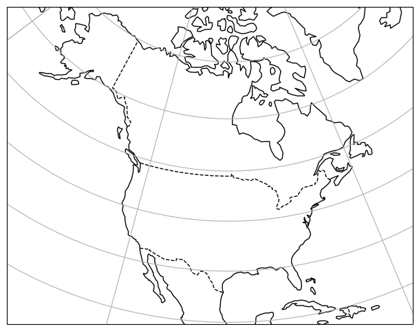
ax = plt.axes(projection=ccrs.LambertConformal())
ax.set_extent([-140, -60, 15, 75], ccrs.Geodetic())
ax.coastlines(); ax.gridlines();
ax.add_feature(cartopy.feature.BORDERS, linestyle='--');

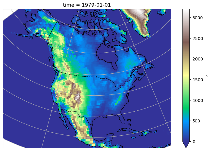
Make a plot

ax = plt.axes(projection=ccrs.LambertConformal())
ax.set_extent([-140, -60, 15, 75], ccrs.PlateCarree())
ax.coastlines();
ax.gridlines();
ax.add_feature(cartopy.feature.BORDERS, linestyle='--');
z.plot(ax=ax, transform=ccrs.PlateCarree(), vmin=0, cmap='terrain');

OK, you should be good now!

Tired of writing so many lines?

Note that it is possible to simplify your plotting commands by writing a function:

def prepare_plot(figsize=None):
    """This function returns prepared axes for the regional plot.
    
    Usage:
        fig, ax = prepare_plot()
    """
    fig = plt.figure(figsize=figsize)
    ax = plt.axes(projection=ccrs.LambertConformal())
    ax.set_extent([-140, -60, 15, 75], ccrs.PlateCarree())
    ax.coastlines(); ax.gridlines();
    ax.add_feature(cartopy.feature.BORDERS, linestyle='--');
    return fig, ax

Now, making a plot has become even easier:

fig, ax = prepare_plot()
z.plot(ax=ax, transform=ccrs.PlateCarree(), vmin=0, cmap='terrain');

Need to save the plot for your presentation?

The easiest way is to use “right-click -> save as” on the image in the notebook.

Also, you can save the plot as pdf or png quite easily (examples below). But this might look quite different as the picture on screen sometimes…

fig, ax = prepare_plot()
z.plot(ax=ax, transform=ccrs.PlateCarree(), vmin=0, cmap='terrain');
plt.savefig('topo.pdf')

fig, ax = prepare_plot()
z.plot(ax=ax, transform=ccrs.PlateCarree(), vmin=0, cmap='terrain');
plt.savefig('topo.png')