Lesson 01: Python and Jupyter: a primer#
Download and open this notebook on your laptop, or open it with MyBinder. Feel free to mess around with it, there is always a fresh copy for you to download!
If you haven’t followed my programming class, you might find these introduction videos useful:
First steps#
At first sight the notebook looks like a text editor. Below the toolbar you can see a cell. The default purpose of a cell is to write code:
a = 'Hello'
print(a)
Hello
You can write one or more lines of code in a cell. You can run this code by clicking on the “Play” button from the toolbar. However it is much faster to use the keybord shortcut: [Shift+Enter] (or [Ctrl+Enter] to stay in the cell). Once you have executed a cell, a new cell should appear below. You can also insert cells with the “Insert” menu. Again, it is much faster to learn the keybord shortcut for this: [Ctrl+m] to enter in command mode then press [a] for “above” or [b] for “below”.
You can click on a cell or type [Enter] to edit it. Create a few empty cells above and below the current one and try to create some variables. You can delete a cell by clicking “delete” in the “edit” menu, or you can use the shortcut: [Ctrl+m] to enter in command mode then press [d] for “delete”, two times!
The variables created in one cell can be used (or overwritten) in subsequent cells:
test = 1
This is text
s = 'Hello'
print(s)
Hello
s = s + ' Python!'
# Note that lines starting with # are not executed. These are for comments.
s
'Hello Python!'
Note that I ommited the print commmand above (this is OK if you want to print something at the end of the cell only).
Code Cells#
In code cells, you can write and execute code. The output will appear underneath the cell, once you execute it.
You can execute your code, as already mentioned before, with the keyboard shortcut [Shift+Enter] or press the Run button in the toolbar. Afterwards, the next cell underneath will be selected automatically.
The Cell menu (classic) or Run menu (lab) has a number of menu items for running code in different ways. These includes:
Run and Select Below: Runs the currently selected cell and afterwards selects the cell below. That’s what you get by pressing
[Shift+Enter]Run and Insert Below: Runs the currently selected cell and inserts a new cell below. Press
[Alt+Enter]Run All: Runs all the code cells included in your jupyter-notebook
Run All Above: Runs all the code cells above the cell you currently selected, excluding this one
Run All Below: All below
The normal workflow in a notebook is, then, quite similar to a standard IPython session, with the difference that you can edit cells in-place multiple times until you obtain the desired results, rather than having to rerun separate scripts with the %run command.
Typically, you will work on a computational problem in pieces, organizing related ideas into cells and moving forward once previous parts work correctly. This is much more convenient for interactive exploration than breaking up a computation into scripts that must be executed together, as was previously necessary, especially if parts of them take a long time to run.
Basic Python syntax#
We are now going to go through some python basics. If you follow the programming lecture with me, you can jump directly to Plotting (although some revision is always good as well!).
In python, the case is important:
Var = 2
var = 3
print(Var + var)
5
In python, the indentation is important:
var = 1
  var += 1  # this raises an Error
  Cell In[6], line 2
    var += 1  # this raises an Error
    ^
IndentationError: unexpected indent
Why is it important? Because Python uses whitespace indentation instead of curly braces or keywords to delimit blocks:
if True:
    print("I'm here!")
else:
    print("Am I?")
print("Now I'm there")
I'm here!
Now I'm there
It’s much less typing! Most beginners don’t like Python because of this, but almost everybody ends up agreeing that this is a great idea.
In Python, you can call functions, like for example abs():
abs(-1)
1
If you feel like it, you can even make your own functions:
def square(x):
    # Be carefull: the indentation!!!
    return x**2
And use it afterwards:
square(4)
16
The “import” mechanism in Python#
Some python functions like print() are always available per default: they are called built-in functions. sorted() is another example:
sorted([2, 4, 1, 5, 3])
[1, 2, 3, 4, 5]
However, there are only a few dozens of available built-in functions in python. Definitely not enough to do serious data-crunching and make Python a competitor to Matlab or R. So what?
Python has a particular mechanism to give access to other functions. This is the import mechanism and is one of the greatest strengths of the Python language (just believe me on this one for now).
import numpy
This is called importing a module. With this simple command we have just “imported” the entire Numpy library. This means that the numpy functions are now available to us. For example, numpy’s arange() function can be called like this:
x = numpy.arange(10)
print(x)
[0 1 2 3 4 5 6 7 8 9]
To get an idea of all the new functions available to us, you can write “numpy.” (“numpy” followed by a dot) in a free cell, then type tab (tab is the autocompletion shortcut of ipython, it is very helpful when writing code).
Because writing “numpy.function()” can be time consuming (especially if one uses numpy often), there is the possibility to give an alias to the imported module. The convention for numpy is following:
import numpy as np
Now the functions can be called like this:
x = np.arange(10)
print(x)
[0 1 2 3 4 5 6 7 8 9]
Variables and arrays#
A variable in Python is very similar to a variable in Matlab or in other languages. A variable can be initialised, used and re-initialised:
x = 10
y = x**2
print(y)
y = 'Hi!'
print(y)
100
Hi!
There are several variable types in Python. We are going to need only very few of them:
Numbers: integers and floats#
i = 12
f = 12.5
print(f - i)
0.5
Strings:#
s = 'This is a string.'
s = "This is also a string."
Strings can be concatenated:
answer = '42'
s = 'The answer is: ' + answer
print(s)
The answer is: 42
But:
answer = 42
s = 'The answer is: ' + answer
print(s)  # this will raise a TypeError
---------------------------------------------------------------------------
TypeError                                 Traceback (most recent call last)
Cell In[20], line 2
      1 answer = 42
----> 2 s = 'The answer is: ' + answer
      3 print(s)  # this will raise a TypeError

TypeError: can only concatenate str (not "int") to str
Numbers can be converted to strings like this:
s = 'Pi is equal to ' + str(np.pi)
print(s)
Pi is equal to 3.141592653589793
Or they can be formated at whish:
s = 'Pi is equal to  {:.2f} (approximately).'.format(np.pi) # the {:.2f} means: print the number with two digits precision
print(s)
Pi is equal to 3.14 (approximately).
Lists#
A list is simply a sequence of things:
l = [1, 2, 'Blue', 3.14]
It has a length and can be indexed:
print(len(l))
print(l[2])
4
Blue
Note: in python the indexes start at zero and not at 1 like in Matlab!
Lists are not like Matlab arrays:
l = [1, 2, 'Blue', 3.14] + ['Red', 'Green']  # adding lists together concatenates them
print(l)
[1, 2, 'Blue', 3.14, 'Red', 'Green']
For Matlab-like arrays we will need Numpy:
Arrays#
a = np.array([1, 2, 3, 4])
a
array([1, 2, 3, 4])
Now we can do element-wise operations on them like in matlab:
print(a + 1)
[2 3 4 5]
print(a * 2)
[2 4 6 8]
It is possible to index arrays like lists:
a[2]
3
Or using for example a range of values:
a[1:3] # the index values from 1 (included) to 3 (excluded) are selected
array([2, 3])
a[1:] # the index values from 1 (included) to the end are selected
array([2, 3, 4])
Multidimensional arrays#
In science, most of the data is multidimensional. Numpy (like Matlab) has been designed for such data arrays:
b = np.array([[0, 1, 2, 3], [4, 5, 6, 7]])
b
array([[0, 1, 2, 3],
       [4, 5, 6, 7]])
The shape of an array is simply its dimensions:
print(b.shape)
(2, 4)
The same kind of elementwise arithmetic is possible on multidimensional arrays:
print(b + 1)
[[1 2 3 4]
 [5 6 7 8]]
And indexing:
b[:, 1:3]
array([[1, 2],
       [5, 6]])
Python objects#
In python, all variables are also “things”. In the programming jargon, these “things” are called objects. Without going into details that you won’t need for this lecture, objects have so-called “attributes” and “methods” (what you may know under the name “functions”). Attributes are information stored about the object.
For example, even simple integers are also “things with attributes”:
# Let's define an interger
a = 1
# Get its attributes
print('The real part of a is', a.real)
print('The imaginary part of a is', a.imag)
The real part of a is 1
The imaginary part of a is 0
Attributes are read with a dot. They are very much like variables. In fact, they are variables:
ra = a.real
ra
1
Importantly, objects can also have functions that apply to them. For example, strings have a function called split():
s = 'This:is:a:splitted:example'
s_splitted = s.split(':')
print(s_splitted)
['This', 'is', 'a', 'splitted', 'example']
One difference between attributes and functions is that the functions are called with parentheses, and sometimes they require arguments (the ':' in this case). Another difference between functions and variables is that the function is almost always returning you something back (yes, some functions return nothing, but they are rare).
Strings also have a join() method by the way:
' '.join(s_splitted)
'This is a splitted example'
It is not necessary to know the details about object oriented programming to use python (in fact, most of the time you don’t need to implement these concepts yourselves). But it is important to know that you can have access to attributes and methods on almost everything in python.
As you will see, we are going to use various attributes and methods available on xarray objects starting from Week 02.
Getting help about python variables and functions#
The standard way to get information about python things is to use the built-in function help(). I am not a big fan of it because its output is quite long, but at least it’s complete:
s = 3
help(s)
Help on int object:

class int(object)
 |  int([x]) -> integer
 |  int(x, base=10) -> integer
 |
 |  Convert a number or string to an integer, or return 0 if no arguments
 |  are given.  If x is a number, return x.__int__().  For floating point
 |  numbers, this truncates towards zero.
 |
 |  If x is not a number or if base is given, then x must be a string,
 |  bytes, or bytearray instance representing an integer literal in the
 |  given base.  The literal can be preceded by '+' or '-' and be surrounded
 |  by whitespace.  The base defaults to 10.  Valid bases are 0 and 2-36.
 |  Base 0 means to interpret the base from the string as an integer literal.
 |  >>> int('0b100', base=0)
 |  4
 |
 |  Built-in subclasses:
 |      bool
 |
 |  Methods defined here:
 |
 |  __abs__(self, /)
 |      abs(self)
 |
 |  __add__(self, value, /)
 |      Return self+value.
 |
 |  __and__(self, value, /)
 |      Return self&value.
 |
 |  __bool__(self, /)
 |      True if self else False
 |
 |  __ceil__(...)
 |      Ceiling of an Integral returns itself.
 |
 |  __divmod__(self, value, /)
 |      Return divmod(self, value).
 |
 |  __eq__(self, value, /)
 |      Return self==value.
 |
 |  __float__(self, /)
 |      float(self)
 |
 |  __floor__(...)
 |      Flooring an Integral returns itself.
 |
 |  __floordiv__(self, value, /)
 |      Return self//value.
 |
 |  __format__(self, format_spec, /)
 |      Convert to a string according to format_spec.
 |
 |  __ge__(self, value, /)
 |      Return self>=value.
 |
 |  __getattribute__(self, name, /)
 |      Return getattr(self, name).
 |
 |  __getnewargs__(self, /)
 |
 |  __gt__(self, value, /)
 |      Return self>value.
 |
 |  __hash__(self, /)
 |      Return hash(self).
 |
 |  __index__(self, /)
 |      Return self converted to an integer, if self is suitable for use as an index into a list.
 |
 |  __int__(self, /)
 |      int(self)
 |
 |  __invert__(self, /)
 |      ~self
 |
 |  __le__(self, value, /)
 |      Return self<=value.
 |
 |  __lshift__(self, value, /)
 |      Return self<<value.
 |
 |  __lt__(self, value, /)
 |      Return self<value.
 |
 |  __mod__(self, value, /)
 |      Return self%value.
 |
 |  __mul__(self, value, /)
 |      Return self*value.
 |
 |  __ne__(self, value, /)
 |      Return self!=value.
 |
 |  __neg__(self, /)
 |      -self
 |
 |  __or__(self, value, /)
 |      Return self|value.
 |
 |  __pos__(self, /)
 |      +self
 |
 |  __pow__(self, value, mod=None, /)
 |      Return pow(self, value, mod).
 |
 |  __radd__(self, value, /)
 |      Return value+self.
 |
 |  __rand__(self, value, /)
 |      Return value&self.
 |
 |  __rdivmod__(self, value, /)
 |      Return divmod(value, self).
 |
 |  __repr__(self, /)
 |      Return repr(self).
 |
 |  __rfloordiv__(self, value, /)
 |      Return value//self.
 |
 |  __rlshift__(self, value, /)
 |      Return value<<self.
 |
 |  __rmod__(self, value, /)
 |      Return value%self.
 |
 |  __rmul__(self, value, /)
 |      Return value*self.
 |
 |  __ror__(self, value, /)
 |      Return value|self.
 |
 |  __round__(...)
 |      Rounding an Integral returns itself.
 |
 |      Rounding with an ndigits argument also returns an integer.
 |
 |  __rpow__(self, value, mod=None, /)
 |      Return pow(value, self, mod).
 |
 |  __rrshift__(self, value, /)
 |      Return value>>self.
 |
 |  __rshift__(self, value, /)
 |      Return self>>value.
 |
 |  __rsub__(self, value, /)
 |      Return value-self.
 |
 |  __rtruediv__(self, value, /)
 |      Return value/self.
 |
 |  __rxor__(self, value, /)
 |      Return value^self.
 |
 |  __sizeof__(self, /)
 |      Returns size in memory, in bytes.
 |
 |  __sub__(self, value, /)
 |      Return self-value.
 |
 |  __truediv__(self, value, /)
 |      Return self/value.
 |
 |  __trunc__(...)
 |      Truncating an Integral returns itself.
 |
 |  __xor__(self, value, /)
 |      Return self^value.
 |
 |  as_integer_ratio(self, /)
 |      Return a pair of integers, whose ratio is equal to the original int.
 |
 |      The ratio is in lowest terms and has a positive denominator.
 |
 |      >>> (10).as_integer_ratio()
 |      (10, 1)
 |      >>> (-10).as_integer_ratio()
 |      (-10, 1)
 |      >>> (0).as_integer_ratio()
 |      (0, 1)
 |
 |  bit_count(self, /)
 |      Number of ones in the binary representation of the absolute value of self.
 |
 |      Also known as the population count.
 |
 |      >>> bin(13)
 |      '0b1101'
 |      >>> (13).bit_count()
 |      3
 |
 |  bit_length(self, /)
 |      Number of bits necessary to represent self in binary.
 |
 |      >>> bin(37)
 |      '0b100101'
 |      >>> (37).bit_length()
 |      6
 |
 |  conjugate(...)
 |      Returns self, the complex conjugate of any int.
 |
 |  is_integer(self, /)
 |      Returns True. Exists for duck type compatibility with float.is_integer.
 |
 |  to_bytes(self, /, length=1, byteorder='big', *, signed=False)
 |      Return an array of bytes representing an integer.
 |
 |      length
 |        Length of bytes object to use.  An OverflowError is raised if the
 |        integer is not representable with the given number of bytes.  Default
 |        is length 1.
 |      byteorder
 |        The byte order used to represent the integer.  If byteorder is 'big',
 |        the most significant byte is at the beginning of the byte array.  If
 |        byteorder is 'little', the most significant byte is at the end of the
 |        byte array.  To request the native byte order of the host system, use
 |        `sys.byteorder' as the byte order value.  Default is to use 'big'.
 |      signed
 |        Determines whether two's complement is used to represent the integer.
 |        If signed is False and a negative integer is given, an OverflowError
 |        is raised.
 |
 |  ----------------------------------------------------------------------
 |  Class methods defined here:
 |
 |  from_bytes(bytes, byteorder='big', *, signed=False)
 |      Return the integer represented by the given array of bytes.
 |
 |      bytes
 |        Holds the array of bytes to convert.  The argument must either
 |        support the buffer protocol or be an iterable object producing bytes.
 |        Bytes and bytearray are examples of built-in objects that support the
 |        buffer protocol.
 |      byteorder
 |        The byte order used to represent the integer.  If byteorder is 'big',
 |        the most significant byte is at the beginning of the byte array.  If
 |        byteorder is 'little', the most significant byte is at the end of the
 |        byte array.  To request the native byte order of the host system, use
 |        `sys.byteorder' as the byte order value.  Default is to use 'big'.
 |      signed
 |        Indicates whether two's complement is used to represent the integer.
 |
 |  ----------------------------------------------------------------------
 |  Static methods defined here:
 |
 |  __new__(*args, **kwargs)
 |      Create and return a new object.  See help(type) for accurate signature.
 |
 |  ----------------------------------------------------------------------
 |  Data descriptors defined here:
 |
 |  denominator
 |      the denominator of a rational number in lowest terms
 |
 |  imag
 |      the imaginary part of a complex number
 |
 |  numerator
 |      the numerator of a rational number in lowest terms
 |
 |  real
 |      the real part of a complex number
A somewhat more user-friendly solution is to use the ? operator provided by the notebook:
s?
You can also ask for help about functions. Let’s ask what numpy’s arange is doing:
np.arange?
I personally don’t use these tools often, because most of the time they don’t provide examples on how to do things. They are useful mostly if you would like to know how the arguments of a function are named, or what a variable is. Especially in the beginning, the best help you can get is with a search machine and especially on the documentation pages of the libraries we are using. This semester, we are going to rely mostly on three components:
numpy: this is the base on which any scientific python project is built.
matplotlib: plotting tools
xarray: working with multidimensional data
It’s always useful to have their documentation webpage open on your browser for easy reference.
Plotting#
The most widely used plotting tool for Python is Matplotlib. Its syntax is directly inspired from Matlab so you should be able to recognise some commands. First, import it:
import matplotlib.pyplot as plt
Don’t worry about why we’ve imported “matplotlib.pyplot” and not just “matplotlib”, this is not important.
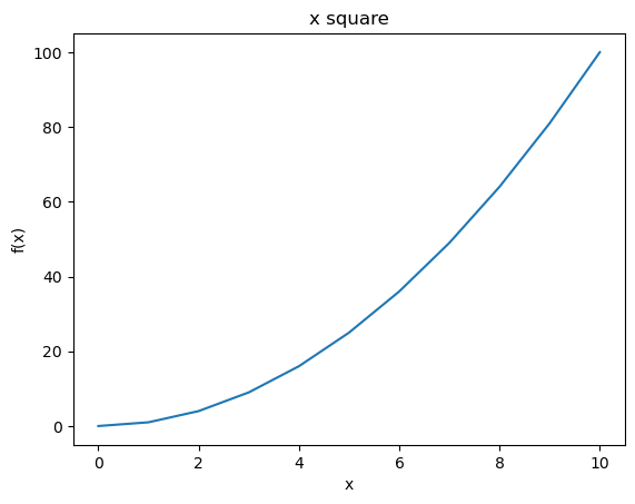
Now we will plot the function \(f(x) = x^2\):
x = np.arange(11)
plt.plot(x, x**2)
plt.xlabel('x')
plt.ylabel('f(x)')
plt.title('x square');  # the semicolon (;) is optional. Try to remove it and see what happens
It is possible to save the figure to a file by adding for example plt.savefig('test.png') at the end of the cell. This will create an image file in the same directory as the notebook.
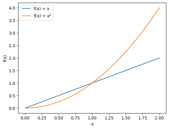
We can also make a plot with several lines and a legend, if needed:
x = np.linspace(0, 2)
plt.plot(x, x, label='f(x) = x')
plt.plot(x, x**2, label='f(x) = x$^{2}$')
plt.xlabel('x')
plt.ylabel('f(x)')
plt.legend(loc='best');
Formatting your notebook with text, titles and formulas.#
The default role of a cell is to run code, but you can tell the notebook to format a cell as “text” by clicking on “Cell \(\rightarrow\) Cell Type \(\rightarrow\) Markdown”. The current cell will now be transformed to a normal text. Try it out in your testing notebook.
Again, there is a shortcut for this: press [ctrl+m] to enter in command mode and then press [m] for “markdown”.
A text cell can also be a title if you add one or more # at the begining#
A text cell can be formatted using the Markdown format. No need to learn too many details about it right now but remember that it is possible to write lists:
item 1
item 2
or formulas:
I can also write text in bold or cursive, and inline formulas: \(i^2 = -1\).
The markdown “code” of this cell is:
A text cell can be formatted using the [Markdown](https://en.wikipedia.org/wiki/Markdown) format.
No need to learn too many details about it right now but remember that it is possible to write lists:
- item 1
- item 2

or formulas:

$$ E = m c^2$$

I can also write text in **bold** or *cursive*, and inline formulas: $i^2 = -1$.

The markdown "`code`" of this cell is:
You can also link to images online (this needs internet to display!) or locally with a path:

Source: http://edu.oggm.org
Useful notebook shortcuts#
Keyboard shortcuts will make your life much easier when using notebooks. To be able to use those shortcuts, you will first need to get into the so called command mode by pressing esc. You will also enter this mode, if you single click on a cell. The color of the cells left margin will turn from green (edit mode) to blue.
Now you can
Switch your cell between code and markdown: press
[m]to markdown and[y]to code.Add a cell: press
[b]to add a cell below,[a]to add one above.Delete a cell: double-press
[d].Move up/down:
[k]/[j]or[arrow up]/[arrow down]Cut/Copy/paste cells:
[x]/[c]/[v]Select multiple cells (lab only):
shift+up/down arrowsInterrupt a computation: double-press
[i].
If you are currently in command mode and want to change back to the edit mode, in which you can edit the text or code of your cells, just press enter or double click on the cell you want to edit.
If you want to execute/run your cell of code or text, press shift + enter. If it was a cell of python code, the output will appear underneath.
The Help->Keyboard Shortcuts dialog lists all the available shortcuts.
What’s next?#
We have learned about the very basics of the python language and the jupyter notebook, and this will be enough for today’s excercises. You can learn more about the notebook by clicking on the “Help” menu above.
There is an excellent Python tutorial provided by the Software Carpentry: http://swcarpentry.github.io/python-novice-inflammation. I strongly recommend it.
If you are ready to go further, let’s go to this week’s lesson and exercises!