Lesson: working with netCDF data#

Last week you learned how to use the basic features of the python language with the numpy and matplotlib libraries. The purpose of this lesson is to introduce you to the main tool that you will use in the semester: xarray.

This is a dense lesson. Please do it entirely and try to remember its structure and content. This code will provide a template for your own code, and you can always come back to these examples when you’ll need them. I don’t expect you to understand all details, but I hope that you are going to get acquainted with the “xarray way” of manipulating multi-dimensional data. You will have to copy and adapt parts of the code below to complete the exercises.

Remember that I will never ask you to use tools you didn’t use in a lesson before! If this happens it was a mistake from my side, sorry!

A first plot#

2d data#

We are now going to plot the average Top of The Atmosphere Shortwave Flux on a map:

# Define the map projection (how does the map look like)
ax = plt.axes(projection=ccrs.EqualEarth())
# ax is an empty plot. We now plot the variable sw_avg onto ax
sw_avg.plot(ax=ax, transform=ccrs.PlateCarree()) 
# the keyword "transform" tells the function in which projection the data is stored 
ax.coastlines(); ax.gridlines(); # Add gridlines and coastlines to the plot

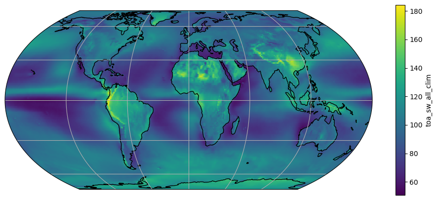
../_images/01_Lesson_NetCDF_Data_47_0.png

We are looking at the average TOA outgoing shorwage flux, expressed in W m\(^{-2}\). Such time averages are often writen with a bar on top of them:

\(\overline{SW_{TOA}} = temporal\_mean(SW_{TOA})\)

Q: look at the basic features of the plot. Can you explain most of the patterns that you observe? Where are the highest values? The lowest ones?

1d data#

It is equally easy to plot 1d data. In this case, we are going to compute the zonal average of sw_avg. “Zonal average” means “along a latitude circle”. It is often writen with [] or <> in formulas:

\(\left[ \overline{SW_{TOA}} \right] = zonal\_mean(temporal\_mean(SW_{TOA}))\)

Note that the two operators are commutative, i.e.:

\(\left[ \overline{SW_{TOA}} \right] = \overline{\left[ SW_{TOA} \right]}\)

Let’s compute it and plot it right away:

sw_avg.mean(dim='lon').plot();

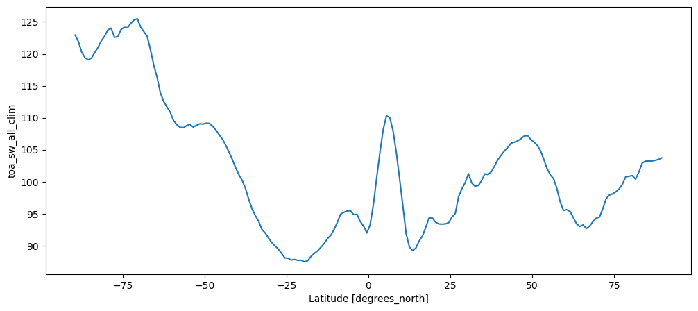
../_images/01_Lesson_NetCDF_Data_52_0.png

Q: look at the basic features of the plot. Can you recognize the important features from the map above?

More data manipulation with xarray#

As you have probably noted already, xarray’s objects (called Dataset for the whole netCDF file or DataArray for single variables) are quite powerful, and can do more than much arrays know from other languages. Last week we talked about the differences between python’s lists and numpy’s arrays. Today we introduced this new object (DataArray) which is one level higher in usability.

But don’t worry if this sounds confusing at first! From now on we are going to use DataArrays only. The best thing about them is that they carry their dimension names and coordinates with them. This is the reason why it was so easy to make a plot with the right axis labels in just one command. They have very useful other properties, and we will learn these step by step.

One of the first nice properties is that they behave just like regular arrays. That is, you can do arithmetic with them. Our first task will be to compute the net energy balance at the top of the atmosphere:

\[\overline{EB_{TOA}} = \overline{SW_{In}} - \overline{SW_{TOA}} - \overline{LW_{TOA}} \approx 0\]

Arithmetics and averages on a sphere#

# Note that there are many different ways to get to the same result. For the sake of clarity we use the simple way:
eb_avg = ds.solar_clim.mean(dim='month') - ds.toa_sw_all_clim.mean(dim='month') - ds.toa_lw_all_clim.mean(dim='month')

E: plot eb_avg on a map. Why did xarray use another colormap? Describe the basic features of the plot. Where is the climate system gaining energy? Losing energy?

# your answer here

We said that the energy balance should be close to zero (balanced). Fortunately, it is easy to check:

eb_avg.mean().item()

-28.665794372558594

But, wait? This is quite far from zero!!! What’s going on here?

Well, it’s simpler than it seems. This is an anoying problem with our planet: it happens to be a sphere. (Or something close to a sphere).

So when we average without taking this into account, we get wrong results. How wrong is it? A regular plot of the data will help us to see what happens here:

eb_avg.plot();

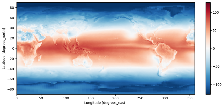
../_images/01_Lesson_NetCDF_Data_63_0.png

Which has to be compared to a sphere. When averaging [lon, lat] data, one gives too much weight to high latitudes.

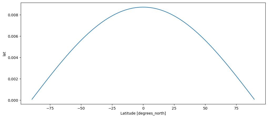
Fortunately, this can be solved by noting that we have to weight each latitudinal band by the cosinus of the latitude, i.e. \(\cos \varphi\). We are going to compute a new average, but weighted this time. First, let’s make a weight array:

weight = np.cos(np.deg2rad(ds.lat))
weight = weight / weight.sum()

weight.plot();

../_images/01_Lesson_NetCDF_Data_66_0.png

Q: can you follow each step? If not, redo each step one by one, and use the ? to get help about each of these functions!

# your answer here

Weight is an array of 180 elements, which is normalised so that it’s sum is 1. This is exactly what we need to compute a weighted average! First, we have to average over the longitudes (this is fine, because along a latitude circle all points have the same weight), and then compute the weighted average.

zonal_eb_avg = eb_avg.mean(dim='lon')  # important! Always average over longitudes first
# this averaging is needed so that the arithmetic below makes sense 
# (multiply two arrays of 180 elements together)
weighted_eb_avg = np.sum(zonal_eb_avg * weight)
weighted_eb_avg.item()

0.9690554141998291

Aaaah, this looks much better now. Not exactly zero, but much closer.

Note: the remaining value (called the residual) is a combination of measurement errors, geometrical approximations (the Earth is not a perfect sphere, see e.g. this post for a more correct implementation which yields ~1.07 instead of 0.97), and anthropogenic energy imbalance (refs 1, 2).

Data selection and multiline plots#

We have seen that DataArrays can be averaged along one dimension as follows:

eb_lon_avg = ds.solar_clim.mean(dim='lon')
eb_lon_avg

<xarray.DataArray 'solar_clim' (month: 12, lat: 180)>
array([[495.7     , 495.60004 , 495.2822  , ...,   0.      ,   0.      ,
          0.      ],
       [306.      , 305.89996 , 305.69998 , ...,   0.      ,   0.      ,
          0.      ],
       [ 59.189995,  60.143776,  62.062664, ...,  22.60511 ,  20.660666,
         19.69    ],
       ...,
       [212.1     , 212.      , 211.9     , ...,   0.      ,   0.      ,
          0.      ],
       [440.7     , 440.5     , 440.28442 , ...,   0.      ,   0.      ,
          0.      ],
       [549.10004 , 549.      , 548.6267  , ...,   0.      ,   0.      ,
          0.      ]], dtype=float32)
Coordinates:
  * lat      (lat) float32 -89.5 -88.5 -87.5 -86.5 -85.5 ... 86.5 87.5 88.5 89.5
  * month    (month) int32 1 2 3 4 5 6 7 8 9 10 11 12

xarray.DataArray

'solar_clim'

month: 12
lat: 180

495.7 495.6 495.3 494.8 494.2 493.5 492.5 ... 0.0 0.0 0.0 0.0 0.0 0.0

array([[495.7     , 495.60004 , 495.2822  , ...,   0.      ,   0.      ,
          0.      ],
       [306.      , 305.89996 , 305.69998 , ...,   0.      ,   0.      ,
          0.      ],
       [ 59.189995,  60.143776,  62.062664, ...,  22.60511 ,  20.660666,
         19.69    ],
       ...,
       [212.1     , 212.      , 211.9     , ...,   0.      ,   0.      ,
          0.      ],
       [440.7     , 440.5     , 440.28442 , ...,   0.      ,   0.      ,
          0.      ],
       [549.10004 , 549.      , 548.6267  , ...,   0.      ,   0.      ,
          0.      ]], dtype=float32)

Coordinates: (2)

lat

(lat)

float32

-89.5 -88.5 -87.5 ... 88.5 89.5

long_name :: Latitude
standard_name :: latitude
units :: degrees_north
valid_range :: [-90. 90.]

array([-89.5, -88.5, -87.5, -86.5, -85.5, -84.5, -83.5, -82.5, -81.5, -80.5,
       -79.5, -78.5, -77.5, -76.5, -75.5, -74.5, -73.5, -72.5, -71.5, -70.5,
       -69.5, -68.5, -67.5, -66.5, -65.5, -64.5, -63.5, -62.5, -61.5, -60.5,
       -59.5, -58.5, -57.5, -56.5, -55.5, -54.5, -53.5, -52.5, -51.5, -50.5,
       -49.5, -48.5, -47.5, -46.5, -45.5, -44.5, -43.5, -42.5, -41.5, -40.5,
       -39.5, -38.5, -37.5, -36.5, -35.5, -34.5, -33.5, -32.5, -31.5, -30.5,
       -29.5, -28.5, -27.5, -26.5, -25.5, -24.5, -23.5, -22.5, -21.5, -20.5,
       -19.5, -18.5, -17.5, -16.5, -15.5, -14.5, -13.5, -12.5, -11.5, -10.5,
        -9.5,  -8.5,  -7.5,  -6.5,  -5.5,  -4.5,  -3.5,  -2.5,  -1.5,  -0.5,
         0.5,   1.5,   2.5,   3.5,   4.5,   5.5,   6.5,   7.5,   8.5,   9.5,
        10.5,  11.5,  12.5,  13.5,  14.5,  15.5,  16.5,  17.5,  18.5,  19.5,
        20.5,  21.5,  22.5,  23.5,  24.5,  25.5,  26.5,  27.5,  28.5,  29.5,
        30.5,  31.5,  32.5,  33.5,  34.5,  35.5,  36.5,  37.5,  38.5,  39.5,
        40.5,  41.5,  42.5,  43.5,  44.5,  45.5,  46.5,  47.5,  48.5,  49.5,
        50.5,  51.5,  52.5,  53.5,  54.5,  55.5,  56.5,  57.5,  58.5,  59.5,
        60.5,  61.5,  62.5,  63.5,  64.5,  65.5,  66.5,  67.5,  68.5,  69.5,
        70.5,  71.5,  72.5,  73.5,  74.5,  75.5,  76.5,  77.5,  78.5,  79.5,
        80.5,  81.5,  82.5,  83.5,  84.5,  85.5,  86.5,  87.5,  88.5,  89.5],
      dtype=float32)

month
(month)
int32
1 2 3 4 5 6 7 8 9 10 11 12
long_name :
Climatological Monthly Means Based on 07/2005 to 06/2015
standard_name :
climatology time
climatology :
climatology_bounds
units :
months of a climatology year
delta_t :
0000-01-00 00:00:00
```
array([ 1,  2,  3,  4,  5,  6,  7,  8,  9, 10, 11, 12], dtype=int32)
```

Attributes: (0)

The resulting array has dimensions (month, lat). A common thing we like to do is for example select certain months, this is an easy task with xarray and the method .sel():

avg_jan = eb_lon_avg.sel(month=1)

E: plot avg_jan to make sure that it is indeed what you think it is.

# your answer here

With the help of a few commands, it is not a big deal to make a nice looking plot:

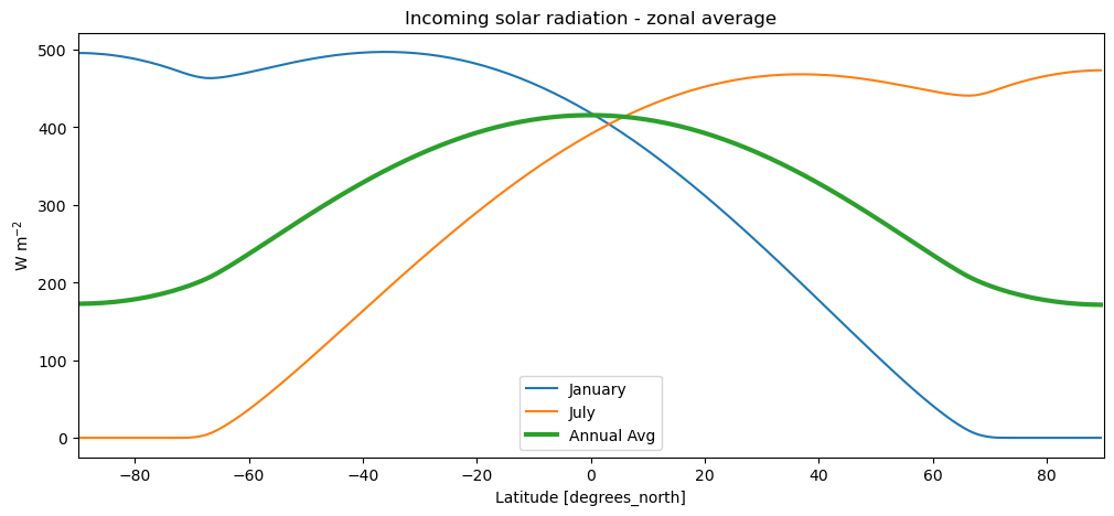
eb_lon_avg.sel(month=1).plot(label='January')
eb_lon_avg.sel(month=7).plot(label='July')
eb_lon_avg.mean(dim='month').plot(label='Annual Avg', linewidth=3)
plt.xlim(-90, 90)
plt.title('Incoming solar radiation - zonal average')
plt.legend(loc='best')
plt.ylabel('W m$^{-2}$');

../_images/01_Lesson_NetCDF_Data_80_0.png

Physics of the Climate System

Lesson: working with netCDF data

Contents

Lesson: working with netCDF data#

NetCDF Files#

Imports and options#

Get the data#

Read the data#

Coordinates#

Variables#

Simple analyses#