
TL;DR
Since this blog post is now one of the top web search results for “WRF projection”, I thought it’d be good to summarize the most important points. Here they are:
- all you need to know about the WRF projection parameters is found in the WRF netcdf file output
- you can plot WRF output with python very easily thanks to the WRF-Python or salem packages
- if you need to parse the projection parameters yourself: don’t forget to adjust the
semimajor_axisandsemiminor_axisprojection parameters to 6370000 (sphere)
If you want know more, read further…
Last week I had to sneak into a conversation between ACINN researchers about how to plot the output of the Weather Research and Forecasting model on a map. This question might seem trivial but it actually isn’t. In fact, the map projection of WRF is so special that some scientists at NCAR wrote a paper about it. They write that geolocalisation errors can lead to “[…] discrepancies that can exceed 20 km at midlatitudes. […] Concurrently, the modeling community should update preprocessing systems to make sure input data are correctly mapped for all global and limited-area simulation domains.”
The paper shows that these discrepancies can have a dramatic effect. However, the paper can be misleading at first sight: WRF users could interpret the paper as an incentive to compute a datum shift between the standard WGS84 ellipsoid and the spherical Earth used by the model. In fact, you shouldn’t: the WRF default terrain and land-cover data are all in provided in the standard WGS84 Datum. This paper (and another surprisingly similar one) actually argue that the input data should also be transformed in a spherical coordinate system before being used by WRF. I think that this would make things even more complex, so we should rather put this problem aside for now.
Uh? You lost me already
Yes, I know - I don’t get it either. If you want to stop reading now, just remember this: use the WRF spherical earth radius parameters to define the WRF map projection, and consider the lon/lat coordinates obtained this way as being valid in WGS84.
Want to read further?
OK, let’s go back a few steps…
… and try to understand how the WRF projection works. If you google a little bit you’ll find many posts the subject. From all these information, I particularly like this illustration by Pavel Krč:
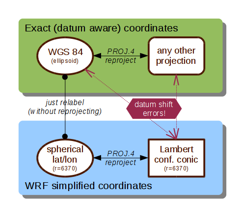
The figure makes three points:
- a classical transformation between two map projections requires three steps: (1) the conversion of eastings/northings to lons/lats, (2) a datum shift, and (3) convert back the lons/lats to eastings/northings
- you have to use the radius of the WRF sphere to define the WRF map projection (in this example Lambert Conformal Conic, but it’s also true for Mercator or Polar projections)
- the lon/lat coordinates obtained from the conversion of the spherical WRF eastings/northings need to be interpreted a being in the standard WGS84 datum, not as spherical lon/lat. Therefore no datum shift is required!
How do I apply this to my WRF file?
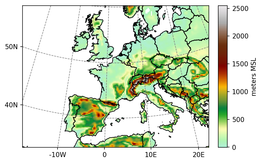
In practice, it’s relatively simple. Let’s open a stantard WRF geogrid file and plot it with our favorite library:
import salem
ds = salem.open_wrf_dataset('geo_em.d01.nc')
ds.HGT_M.where(ds.LANDMASK).salem.quick_map(cmap='topo');
Now, although salem would do all the job for you, let’s try to get the projection right without external help. The projection parameters are stored as attributes in the NetCDF file:
import pyproj
wrf_proj = pyproj.Proj(proj='lcc', # projection type: Lambert Conformal Conic
                       lat_1=ds.TRUELAT1, lat_2=ds.TRUELAT2, # Cone intersects with the sphere
                       lat_0=ds.MOAD_CEN_LAT, lon_0=ds.STAND_LON, # Center point
                       a=6370000, b=6370000) # This is it! The Earth is a perfect sphere
Now, how do we now that we got it right? The best test is to see if we are able to re-compute the lons and lats that WRF provides in the original files:
# Easting and Northings of the domains center point
wgs_proj = pyproj.Proj(proj='latlong', datum='WGS84')
e, n = pyproj.transform(wgs_proj, wrf_proj, ds.CEN_LON, ds.CEN_LAT)
# Grid parameters
dx, dy = ds.DX, ds.DY
nx, ny = ds.dims['west_east'], ds.dims['south_north']
# Down left corner of the domain
x0 = -(nx-1) / 2. * dx + e
y0 = -(ny-1) / 2. * dy + n
# 2d grid
xx, yy = np.meshgrid(np.arange(nx) * dx + x0, np.arange(ny) * dy + y0)
xx and yy are the 2D coordinates of each WRF grid point in units of
meters (eastings and northings in the WRF map projection). The computation
of the domain’s center point is not required for the first WRF domain (it is
always centered in its own projection) but it is required for the child domains
(which can be placed anywhere in the map). Let’s convert them to lons and lats
and see how they compare to the original WRF ones:
# Transform and plot
our_lons, our_lats = pyproj.transform(wrf_proj, wgs_proj, xx, yy)
ds['DIFF'] = np.sqrt((our_lons - ds.XLONG_M)**2 + (our_lats - ds.XLAT_M)**2)
ds.salem.quick_map('DIFF', cmap='Reds');

Our lons and lats agree with WRF up to 5 digits after the comma. Now, what would happen if we forget to specify that we are on a sphere, and use the default wgs84 ellipsoid instead?
bad_proj = pyproj.Proj(proj='lcc', # projection type: Lambert Conformal Conic
                       lat_1=ds.TRUELAT1, lat_2=ds.TRUELAT2, # Cone intersects with the sphere
                       lat_0=ds.MOAD_CEN_LAT, lon_0=ds.STAND_LON, # Center point
                       ) # The Earth is now an ellipsoid
bad_lons, bad_lats = pyproj.transform(bad_proj, wgs_proj, xx, yy)
ds['DIFF2'] = np.sqrt((bad_lons - ds.XLONG_M)**2 + (bad_lats - ds.XLAT_M)**2)
print('The max diff is: {}'.format(ds['DIFF2'].max().values))
The max diff is: 0.114...
We have an error of more than 0.1°! It’s even more illustrative to compute the error in meters. We just invert the procedure:
bad_xx, bad_yy = pyproj.transform(wgs_proj, bad_proj, ds.XLONG_M.values, ds.XLAT_M.values)
ds['DIFF_M'] = np.sqrt((bad_xx - xx)**2 + (bad_yy - yy)**2) + ds.XLONG_M*0 # trick
ds.salem.quick_map('DIFF_M', cmap='Reds');

The error in geolocalisation is close to zero in the center and rises up to 7km in the upper corners of the domain.
OK… But why should I care?
You don’t have to care about this if you only use the longitudes and latitudes provided by WRF to do your analysis. They are valid in the WGS84 datum and therefore can be used to find the nearest grid point to a weather station, for example.
For all other applications, you should care.
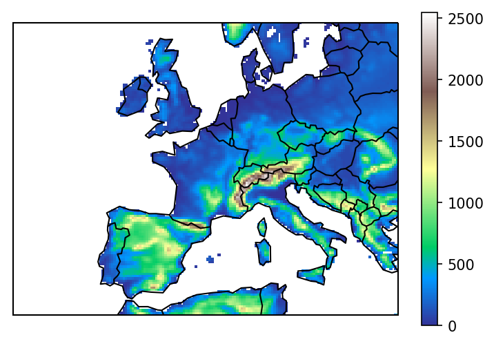
Example plot with cartopy
import cartopy
import cartopy.crs as ccrs
# Define the projection
globe = ccrs.Globe(ellipse='sphere', semimajor_axis=6370000, semiminor_axis=6370000)
lcc = ccrs.LambertConformal(globe=globe, # important!
                            central_longitude=ds.STAND_LON, central_latitude=ds.MOAD_CEN_LAT,
                            standard_parallels=(ds.TRUELAT1, ds.TRUELAT2),
                            )
ax = plt.axes(projection=lcc)
z.plot(ax=ax, transform=lcc, cmap='terrain');
ax.coastlines()
ax.add_feature(cartopy.feature.BORDERS, linestyle='-');
ax.set_extent([xx.min(), xx.max(), yy.min(), yy.max()], crs=lcc)
(note that I don’t show an example with basemap, for two reasons: I don’t know basemap, and basemap is replaced by cartopy anyway).