Lesson 01: future glacier change#
Glaciers are among the most visible indicators of climate change. Their retreat is well documented across the world, but how do we actually quantify these changes? And how do we use model projections to assess future glacier evolution?
This lesson has two parts:
Lesson 01 (this notebook): getting aquainted with glacier data.
Lesson 02 (the following notebook): getting aquainted with geospatial tools to give you more flexibility in your future projects.
By the end of this lesson, you will:
Learn how to work with OGGM glacier projections in Python.
Understand how to analyze ensemble climate projections instead of relying on a single scenario.
This session is methods-focused—it will equip you with the tools you need before diving into the bigger questions in the assignment: How much will glaciers shrink by 2100? What are the uncertainties? And what does this mean for water availability in glacier-fed regions?
Data and context#
We will use projections of glacier change computed with the OGGM model, developed in Bristol in collaboration with several other universities. OGGM is capable of simulating the evolution of all glaciers worldwide. In this workshop, we will not run the model ourselves but instead use pre-computed outputs for a wide range of possible future climate scenarios. These data are available as part of the OGGM standard projections 1.6.1.
For this workshop, I have prepared a subset of the data for the Rhone basin.
To get started:
Go to the data download page and download the tar file for basin number 6243 (Rhone).
Create a new folder in your
datafolder (e.g.,glaciers) and move the file there.Unpack the tar file—this will create a folder named
6243containing several NetCDF files.
Import the packages#
import numpy as np
import matplotlib.pyplot as plt
import xarray as xr
import pandas as pd
OGGM output is provided in NetCDF files: this is why we will need xarray again!
OGGM output file#
Let’s open one singe file to get started. This is the data for the Rhone basin, the OGGM model is forced with with W5E5 data for 2000-2020, and then with the BCC-CSM2-MR climate model under the scenario ssp126 until 2100. You can ignore the rest of the very long filename!
with xr.open_dataset('../data/glaciers/6243/basin_6243_run_hydro_w5e5_gcm_merged_endyr2100_CMIP6_bc_2000_2019_BCC-CSM2-MR_ssp126.nc') as ds:
    ds = ds.load()  # This is a safer way to open files with xarray - we open the file, load the data, and close the netCDF file
Let’s explore the file together:
ds
<xarray.Dataset> Size: 7MB
Dimensions:            (scenario: 1, gcm: 1, time: 101, rgi_id: 1169,
                        month_2d: 12)
Coordinates:
  * time               (time) float64 808B 2e+03 2.001e+03 ... 2.099e+03 2.1e+03
  * rgi_id             (rgi_id) <U14 65kB 'RGI60-11.01238' ... 'RGI60-11.03820'
    hydro_year         (time) int64 808B 2000 2001 2002 2003 ... 2098 2099 2100
    hydro_month        (time) int64 808B 4 4 4 4 4 4 4 4 4 ... 4 4 4 4 4 4 4 4 4
    calendar_year      (time) int64 808B 2000 2001 2002 2003 ... 2098 2099 2100
    calendar_month     (time) int64 808B 1 1 1 1 1 1 1 1 1 ... 1 1 1 1 1 1 1 1 1
  * month_2d           (month_2d) int64 96B 1 2 3 4 5 6 7 8 9 10 11 12
    calendar_month_2d  (month_2d) int64 96B 1 2 3 4 5 6 7 8 9 10 11 12
  * gcm                (gcm) <U11 44B 'BCC-CSM2-MR'
  * scenario           (scenario) <U6 24B 'ssp126'
    bias_correction    <U12 48B 'bc_2000_2019'
Data variables:
    runoff             (scenario, gcm, time, rgi_id) float32 472kB 6.94e+10 ....
    runoff_monthly     (scenario, gcm, time, month_2d, rgi_id) float32 6MB 0....
    volume             (scenario, gcm, time, rgi_id) float32 472kB 1.624e+09 ...
    area               (scenario, gcm, time, rgi_id) float32 472kB 1.575e+07 ...
Attributes:
    description:    OGGM model output
    oggm_version:   1.6.1.dev26+gf8a1745
    calendar:       365-day no leap
creation_date: 2023-06-05 05:37:08ds.gcm
<xarray.DataArray 'gcm' (gcm: 1)> Size: 44B
array(['BCC-CSM2-MR'], dtype='<U11')
Coordinates:
* gcm (gcm) <U11 44B 'BCC-CSM2-MR'
bias_correction <U12 48B 'bc_2000_2019'
Attributes:
description: used global circulation modelThe structure is quite different from what we’ve seen so far. First of all, there are more coordinates than we are used to. And no lats and lons! At least there is a time coordinate - this at least we are familiar with.
Q: There are four variables - can you name them? And give their dimensions and units?
# Your answer here
Let’s remove the year 2000 - indeed, runoff cannot be computed for the final timestep of data (which consists only of January 2100):
ds = ds.sel(time=slice(2000, 2099))
Glacier per glacier simulations#
The rgi_id coordinate corresponds to the unique identifier for all glaciers in the basin - there are 1169 of them. “RGI” stands for Randolph Glacier Inventory, the reference dataset for glacier outlines. Let’s print these ids:
ds.rgi_id
<xarray.DataArray 'rgi_id' (rgi_id: 1169)> Size: 65kB
array(['RGI60-11.01238', 'RGI60-11.01299', 'RGI60-11.01324', ...,
       'RGI60-11.03818', 'RGI60-11.03819', 'RGI60-11.03820'], dtype='<U14')
Coordinates:
* rgi_id (rgi_id) <U14 65kB 'RGI60-11.01238' ... 'RGI60-11.03820'
bias_correction <U12 48B 'bc_2000_2019'
Attributes:
description: RGI glacier identifierThese are just a list of strings. Should we be interested in plotting the volume evolution of one glacier in particular, we could select it like this:
ds['volume'].sel(rgi_id='RGI60-11.03643').plot(); # This is the Mer de glace glacier near Chamonix
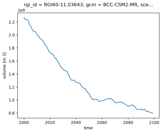
E: now add a new line to the plot for the Argentière glacier nearby (RGI60-11.03638). Then repeat but for the area and runoff variables.
# Your answer here
If you are interested in looking at other glaciers, you can use the GLIMS Glacier Viewer. Here is a tutorial on how to find out the RGI6 ID.
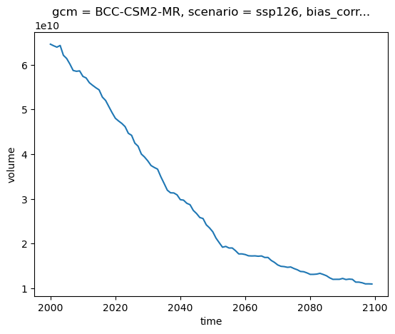
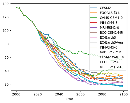
OGGM simulates all the glaciers individually. But for many applications, we want to compute the total volume or runoff in a specific area (here the entire basin). Fortunately, it’s very simple to compute this using xarray:
total_volume = ds.volume.sum(dim='rgi_id')
total_volume.plot();
E: repeat the basin-wide plot for area and runoff.
# Your answer here
Basin-wide volume and area#
The units of m3 are not very practical to use. Often, we will prefer two options to display the data:
km3 is often used instead of m3
instead of absolute change, we will represent % change with respect to a given year. This is the preferred option because we can’t really relate to glacier volume numbers easily.
E: convert the total_volume to km3 and store the output in a new variable (total_volume_km3). Plot it.
# Your answer here
For relative changes, we first have to choose a reference year (for example 2020), and then divide the timeseries by that value. For good measure, we multiply by 100 to obtain percentages:
total_volume_change = (total_volume / total_volume.sel(time=2020)) * 100
total_volume_change.plot();
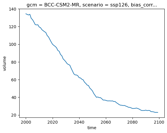
Q: how much volume (in %) did the Rhone basin loose betwen 2000 and 2020? for this GCM and scenario, what is the remaining volume (in %) at the end of the century?
E: now repeat this for basin-wide area.
# Your answer here
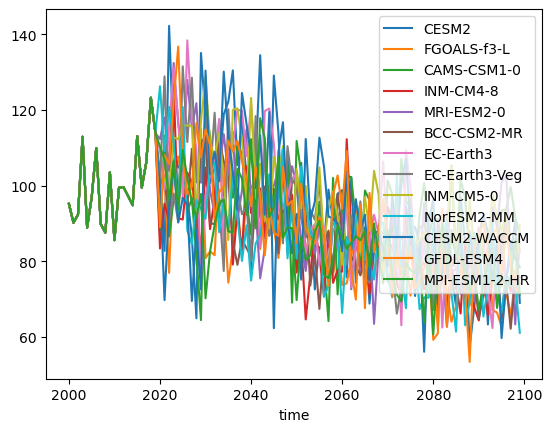
Basin-wide annual runoff#
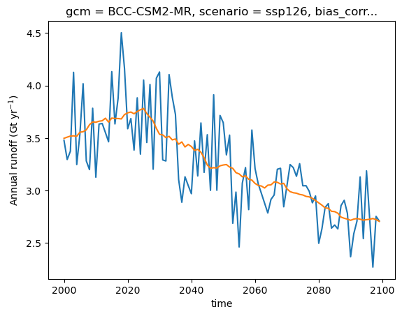
Let’s compute the glacier runoff in gigatons per year:
total_runoff = ds.runoff.sum(dim='rgi_id') * 1e-12  # convert to gigatons
total_runoff.plot();
plt.ylabel('Annual runoff (Gt yr$^{-1}$)');

Glacier runoff in OGGM (and in several other glacier models) is computed as the sum of ice melt, snow melt, and liquid precipitation over the glacier domain. The model follows a temperature-index approach to estimate melt rates. Precipitation and temperature data are provided by W5E5 or a climate model.
In OGGM, runoff is calculated at each time step (monthly or annual) over a fixed spatial domain. This domain corresponds to the total area covered by the glacier at the start of the simulation. When the glacier retreats, OGGM still accounts for snowmelt and liquid precipitation over the newly ice-free area. This is known as a “fixed-gauge” approach, which simplifies comparisons by ensuring that runoff contributions from processes other than glacier melt remain unaffected by glacier retreat.
We will explain glacier runoff in class, but in the meantime, if you’re interested, check out this OGGM tutorial for additional context.
The plot above shows the decreasing glacier contribution to overall runoff, overlaid with interannual variability of melt and precipitation. When studying runoff, it may be useful to compute running averages to smooth out short-term variability and highlight long-term trends:
total_runoff.plot(label='Annual runoff');
total_runoff.rolling(time=21, center=True, min_periods=1).mean().plot(label='21-yr average');
plt.ylabel('Annual runoff (Gt yr$^{-1}$)');
Optional: monthly runoff#
Want to explore how runoff changes throughout the year? Monthly runoff offers a different perspective than annual totals. Just ask me for a “recipe” if you’d like to include this in your project!
The importance of considering ensembles#
Important
The following section is very relevant for any climate risk assessment — not just glaciers. These concepts apply across all climate impact analyses, from floods to crop yields to heatwaves. Please read it carefully and take your time to digest the key ideas.
The projection you see here represents just one realization of future climate conditions, based on a single climate model, a single greenhouse gas scenario, and a specific realization of the climate system’s internal variability. While it provides a coherent story of how the climate might evolve, relying on a single projection can be misleading — it offers no information about the spread, likelihood, or robustness of the result. In decision-making, especially when dealing with climate risk, this is a major problem.
Why is this a problem? Because climate models are inherently uncertain. These uncertainties arise from three main sources:
Internal variability: The climate system is chaotic. Even with the same model and scenario, small changes in initial conditions can lead to different outcomes—especially over the short to medium term.
Model uncertainty: Different climate models make different assumptions about how the Earth system works. They differ in how they simulate clouds, ocean circulation, snow cover, vegetation, aerosols, etc. No single model is “correct” (or, as the famous quote says: “All models are wrong”).
Scenario uncertainty: Future emissions depend on political, economic, and technological developments. Climate models are run under a range of Shared Socioeconomic Pathways (SSPs) to explore this uncertainty.
To address these uncertainties —at least partly— we use multi-model ensembles, such as the CMIP6 ensemble. CMIP (Coupled Model Intercomparison Project) is a coordinated global effort in which climate modeling centers around the world simulate past and future climate under shared scenarios. CMIP6 includes dozens of models run under different SSPs, offering a spread of projections that we can analyze statistically.
By looking at the full ensemble, we can:
Try to better identify the range of possible futures (e.g. temperature or glacier mass in 2100),
Quantify robust changes that are consistent across models (e.g. widespread warming),
Detect outliers or surprises, and
Support risk-based decisions, which depend not only on the most likely outcome but also on low-probability high-impact ones.
We will now use a large CMIP6 ensemble (as available to us) to compute the range of projected future glacier change in the Rhone Basin under the SSP126 scenario. We will explore two different methods to do so.
Note
For a good overview of climate model ensembles and how to interpret them, see:
IPCC AR6 WG1 Chapter 4 (esp. Box 4.1): https://www.ipcc.ch/report/ar6/wg1/chapter/chapter-4/
Method 1: looping over all available files#
import glob

# The * indicates that we allow all kinds of patters here - i.e. all GCMs, but still ssp126
file_pattern = "../data/glaciers/6243/basin_6243_run_hydro_w5e5_gcm_merged_endyr2100_CMIP6_bc_2000_2019_*_ssp126.nc"

# Get all matching files
files = glob.glob(file_pattern)

# Print the list of files
print(f'There are {len(files)} files:')
for f in files:
    print(f)
There are 13 files:
../data/glaciers/6243/basin_6243_run_hydro_w5e5_gcm_merged_endyr2100_CMIP6_bc_2000_2019_CESM2_ssp126.nc
../data/glaciers/6243/basin_6243_run_hydro_w5e5_gcm_merged_endyr2100_CMIP6_bc_2000_2019_FGOALS-f3-L_ssp126.nc
../data/glaciers/6243/basin_6243_run_hydro_w5e5_gcm_merged_endyr2100_CMIP6_bc_2000_2019_CAMS-CSM1-0_ssp126.nc
../data/glaciers/6243/basin_6243_run_hydro_w5e5_gcm_merged_endyr2100_CMIP6_bc_2000_2019_INM-CM4-8_ssp126.nc
../data/glaciers/6243/basin_6243_run_hydro_w5e5_gcm_merged_endyr2100_CMIP6_bc_2000_2019_MRI-ESM2-0_ssp126.nc
../data/glaciers/6243/basin_6243_run_hydro_w5e5_gcm_merged_endyr2100_CMIP6_bc_2000_2019_BCC-CSM2-MR_ssp126.nc
../data/glaciers/6243/basin_6243_run_hydro_w5e5_gcm_merged_endyr2100_CMIP6_bc_2000_2019_EC-Earth3_ssp126.nc
../data/glaciers/6243/basin_6243_run_hydro_w5e5_gcm_merged_endyr2100_CMIP6_bc_2000_2019_EC-Earth3-Veg_ssp126.nc
../data/glaciers/6243/basin_6243_run_hydro_w5e5_gcm_merged_endyr2100_CMIP6_bc_2000_2019_INM-CM5-0_ssp126.nc
../data/glaciers/6243/basin_6243_run_hydro_w5e5_gcm_merged_endyr2100_CMIP6_bc_2000_2019_NorESM2-MM_ssp126.nc
../data/glaciers/6243/basin_6243_run_hydro_w5e5_gcm_merged_endyr2100_CMIP6_bc_2000_2019_CESM2-WACCM_ssp126.nc
../data/glaciers/6243/basin_6243_run_hydro_w5e5_gcm_merged_endyr2100_CMIP6_bc_2000_2019_GFDL-ESM4_ssp126.nc
../data/glaciers/6243/basin_6243_run_hydro_w5e5_gcm_merged_endyr2100_CMIP6_bc_2000_2019_MPI-ESM1-2-HR_ssp126.nc
Now, for each of them, we can extract the volume, and plot it:
for f in files:
    # Extract the GCM name from the file name
    gcm_name = f.split('2000_2019_')[1].split('_ssp')[0]

    # Open and compute
    with xr.open_dataset(f) as ds_tmp:
        ds_tmp = ds_tmp.sel(time=slice(2000, 2099)).load()
        tmp_volume = ds_tmp.volume.sum(dim='rgi_id') * 1e-9

    # Plot
    tmp_volume.plot(label=gcm_name);

plt.legend(); plt.ylabel('Basin volume (km$^3$)'); plt.title('SSP126');
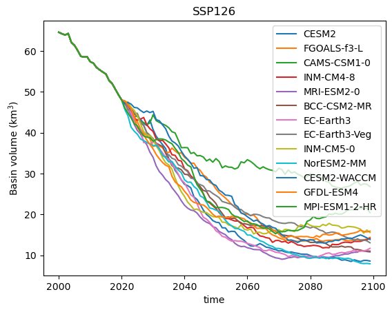
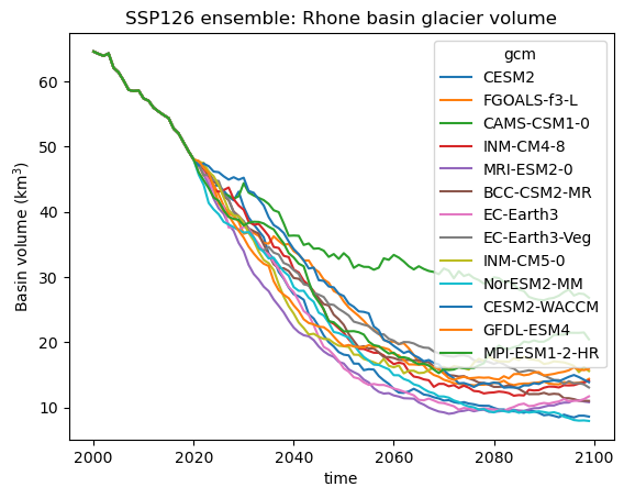
Q: interpret the plot above. Why is the data before 2020 always the same? What is the full range of outcomes for this scenario at the end of the century?
E: Now, instead of computing the absolute volume, compute the relative volume change with respect to 2020, and repeat the plot.
# Your answer here
For a a cleaner workflow, we can store the output of each file in a dataframe instead of reading the files and plotting in the same loop. This is the recommended way for real-life workflows:
# Create the containers
df_runoff = pd.DataFrame()
df_volume = pd.DataFrame()

for f in files:
    # Extract the GCM name from the file name
    gcm_name = f.split('2000_2019_')[1].split('_ssp')[0]

    # Open and compute
    with xr.open_dataset(f) as ds_tmp:
        ds_tmp = ds_tmp.sel(time=slice(2000, 2099)).load()
        tmp_volume = ds_tmp.volume.sum(dim='rgi_id') * 1e-9
        tmp_runoff = ds_tmp.runoff.sum(dim='rgi_id') * 1e-12

    # Store for later
    df_runoff[gcm_name] = tmp_runoff.squeeze().to_series()
    df_volume[gcm_name] = tmp_volume.squeeze().to_series()
Now we have dataframes with with which we can redo the same plots:
df_volume.plot();
df_volume_relative = (df_volume / df_volume.loc[2020]) * 100
df_volume_relative.plot();
For runoff, we prefer to compute the relative runoff with respect to an average period instead of a single year, for example 2000-2019:
df_runoff_relative = (df_runoff / df_runoff.loc[2000:2019].mean()) * 100
df_runoff_relative.plot();
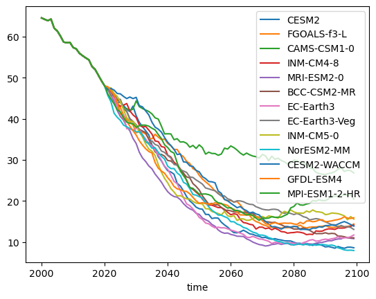
Method 2: open_mf_dataset (optional)#
This will avoid for loops entirely and uses dask for those interested. Ignore the below if you are under time pressure - it’s only important if you want to analyse many files at once.
It requires you to install dask (remember how? conda install -c conda-forge dask (or mamba instead of conda).
# File pattern (same as before)
file_pattern = "../data/glaciers/6243/basin_6243_run_hydro_w5e5_gcm_merged_endyr2100_CMIP6_bc_2000_2019_*_ssp126.nc"

# Get matching files
files = glob.glob(file_pattern)
print(f'Found {len(files)} files.')

# Open all files as a single dataset, adding a new dimension from file name
ds_all = xr.open_mfdataset(
    files,
    combine='nested',
    concat_dim='gcm',
    preprocess=lambda ds: ds.sel(time=slice(2000, 2099)),
    engine='netcdf4'  # or omit if using default
)

# Extract GCM names from filenames
gcm_names = [f.split('2000_2019_')[1].split('_ssp')[0] for f in files]
ds_all['gcm'] = ('gcm', gcm_names)

# Sum volume over all glaciers
volume_by_gcm = ds_all.volume.sum(dim='rgi_id') * 1e-9  # Convert to km³

# Plot spaghetti plot
volume_by_gcm.plot(hue='gcm');
plt.ylabel('Basin volume (km$^3$)')
plt.title('SSP126 ensemble: Rhone basin glacier volume');
Found 13 files.
The advantage of this method is that all data can be handled within xarray without for loops. It also allows to handle extremely large datasets - if you are curious, ask Fabien about it! Otherwise just move on to the next bit:
From “spaghetti” plots to quantiles#
The plot above shows individual model projections of future glacier volume under the SSP126 scenario. Each line represents a different climate model from the CMIP6 ensemble. These are often called “spaghetti plots” because of their overlapping, tangled appearance. While these plots give a sense of the range of possible futures, they can be overwhelming and difficult to interpret. Individual models may show short-term variability that isn’t relevant for long-term trends, and focusing on specific runs may obscure the broader picture of uncertainty.
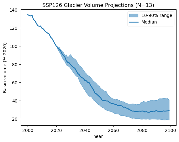
Instead of plotting every model separately, we often summarize projections using quantiles—for example, showing the median (50th percentile), and the spread between the 10th and 90th percentiles.
In the next step, we will compute and visualize these quantile-based ranges to gain a clearer understanding of future glacier runoff trends:
# We compute the quantiles along the ensemble
q10 = df_volume_relative.quantile(0.1, axis=1)
q50 = df_volume_relative.quantile(0.5, axis=1)
q90 = df_volume_relative.quantile(0.9, axis=1)
# Extract the time index from the DataFrame
time = df_volume_relative.index

# Plot the filled quantile range
plt.fill_between(time, q10, q90, color="C0", alpha=0.5, label="10-90% range")

# Plot the median line
plt.plot(time, q50, color="C0", linewidth=2, label="Median")

# Labels and legend
plt.ylabel("Basin volume (% 2020)")
plt.xlabel("Year")
plt.title(f"SSP126 Glacier Volume Projections (N={len(df_volume.columns)})")
plt.legend();
E: now repeat the steps above with with the 0.05 and 0.95 quantiles instead - do you see much difference? Maybe you can even plot both the 10-90% and th 5-95% range on the same plot?
# Your answer here
E: Finally, repeat the 10-90% plot plot with runoff instead of volume.
# Your answer here
Conclusions & next steps: what does glacier change mean?#
In this lesson, we focused on the tools and methods needed to analyze glacier projections:
We opened and processed OGGM projection data.
We examined glacier-wide and basin-wide volume evolution over time.
We explored the importance of climate model ensembles and how to summarize them with quantiles instead of spaghetti plots.
While today was all about data processing, the real question is: What do these projections tell us about future glacier change?
This is where your assignment comes in! You will now take the tools from this lesson and apply them to real-world climate impact questions, such as:
How much glacier volume will be lost by 2100?
How do different climate scenarios (e.g., SSP126 vs. SSP585) affect glacier evolution?
What are the key uncertainties, and how do we interpret them?
Glacier projections are more than just numbers—they are essential for understanding water security, hydrological risks, and long-term climate adaptation strategies. In the next step, you will use your new skills to analyze these impacts and draw meaningful conclusions.