Regridding WorldPop data to your region of choice

I downloaded the global 1km 2020 population product from WorldPop here: https://hub.worldpop.org/doi/10.5258/SOTON/WP00647. Now we will see how we can match these data to another dataset, say for example ERA5 data at 0.25° resolution that I prepared with this script.

# Import the tools we are going to need today:
import matplotlib.pyplot as plt  # plotting library
import numpy as np  # numerical library
import xarray as xr  # netCDF library
import cartopy  # Map projections libary
import cartopy.crs as ccrs  # Projections list

import rioxarray as rioxr  # Open geotiffs with xarray
import xesmf as xe  # Regridder

The key package here is xesmf.

Installing additional packages in an existing environmnent is easy, but only do it if you need a given package!

1. Start by opening a prompt and activating the qcr environment as usual: conda activate qcr

2. Now, install the requested packages. Let’s install a few at a time: type mamba install --channel conda-forge xesmf (or, if mamba is not available, conda install --channel conda-forge xesmf). Answer yes to the questions.

3. That’s it! you can start jupyter-lab as usual.

WorldPop data

Open the data with rasterio, as explained in Workshop 8:

worldpop = rioxr.open_rasterio("../data/worldpop/ppp_2020_1km_Aggregated.tif", masked=True).squeeze()
worldpop = worldpop.rename({'x':'longitude', 'y':'latitude'})  # xesmf wants this

Let’s count how many we are:

f'There were  {worldpop.sum().item() * 1e-9:.1f} billion of us in 2020'

'There were  8.0 billion of us in 2020'

The data is global at 1km resolution, which is quite a lot of data! Let’s select data for West Africa only:

worldpop = worldpop.sel(longitude=slice(-20, 15), latitude=slice(21, 3)).squeeze()

Let’s plot it:

# Define the map projection (how does the map look like)
ax = plt.axes(projection=ccrs.PlateCarree())
# ax is an empty plot. We now plot the variable sw_avg onto ax
worldpop.plot.imshow(ax=ax, transform=ccrs.PlateCarree(), 
                     levels=[1, 10, 50, 100, 500, 1000, 5000],
                     cmap='YlOrRd') 
# the keyword "transform" tells the function in which projection the data is stored 
ax.coastlines(); ax.gridlines(); # Add gridlines and coastlines to the plot
# We set the extent of the map
extent = [worldpop.longitude.min(), worldpop.longitude.max(), 
          worldpop.latitude.min(), worldpop.latitude.max()]
ax.set_extent(extent, crs=ccrs.PlateCarree())

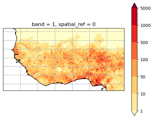
This is the population at 1km resolution.

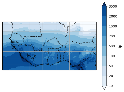
ERA5 data

Let’s open the ERA5 dataset (here precip):

ds = xr.open_dataset('../data/ERA5_WestAfrica/ERA5_LowRes_Monthly_tp.nc')

# Annual precip
annual_prcp = ds.tp.mean(dim='time') * 365.25 * 1000

# Plot it
ax = plt.axes(projection=ccrs.PlateCarree())

annual_prcp.plot(ax=ax, transform=ccrs.PlateCarree(),
                 levels=[10, 20, 50, 100, 500, 700, 1000, 2000, 3000],
                 cmap='Blues') 

ax.coastlines(); ax.gridlines();
ax.add_feature(cartopy.feature.BORDERS, linestyle='--');

extent = [ds.longitude.min(), ds.longitude.max(), ds.latitude.min(), ds.latitude.max()]
ax.set_extent(extent, crs=ccrs.PlateCarree())

Regridding

Regridding is a very common processing step in GIS and climate science. The most frequent step is to resample the high resolution dataset onto the low resolution one.

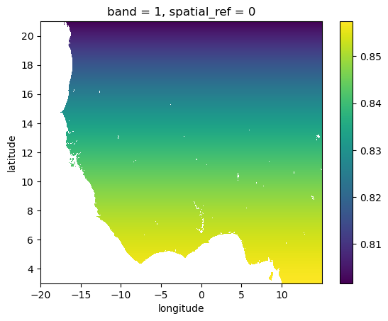
We’ll do this using xesmf. This is normally quite straightforward, but there is one particularity with population data: we are interested in summing, not averaging - xesmf can do only conservative averaginf. Therefore, before regridding, we have to transform population totals in population density instead. Let’s start by computing the area of the worldpop gred cells:

# Define Earth's radius in kilometers
earth_radius_km = 6371  # Earth's radius in km

# Calculate the grid spacing in radians
dx = np.deg2rad(worldpop.longitude[1] - worldpop.longitude[0]) 

# Compute grid cell area in square kilometers
# - dx**2 gives the area in radians squared
# - np.cos(np.deg2rad(worldpop.y)) accounts for latitude-dependent stretching of grid cells
# - Multiplying by earth_radius_km**2 scales the area to square kilometers
worldpop_area_km = earth_radius_km**2 * dx**2 * np.cos(np.deg2rad(worldpop.latitude))

# Expand area to match the full worldpop dataset dimensions
# - worldpop * 0 ensures that the area array has the same shape as worldpop (broadcasting)
# - This is useful when working with multi-dimensional data
worldpop_area_km = worldpop * 0 + worldpop_area_km

# Now worldpop_area_km has the same shape as worldpop and represents the area of each grid cell in km²
worldpop_area_km.plot.imshow();

Now compute the population density (per km2):

worldpop_dens = worldpop / worldpop_area_km

And replace nans with 0s (important! conservative regridding works best with no missing data, and missing data here equals no populations anyways):

worldpop_dens = worldpop_dens.fillna(0)

Regrid the population density:

do_compute = False  # I set it to false because I already computed it
if do_compute:
    # This may take several minutes - I show a trick to make it faster below,
    # but this is the most accurate way
    regridder = xe.Regridder(worldpop_dens, annual_prcp, method='conservative')
    worldpop_dens_on_era5 = regridder(worldpop_dens)
    
    # And convert the population density back to population totals:
    dx_era = np.deg2rad(ds.longitude[1] - ds.longitude[0]) 
    era_area_km = earth_radius_km**2 * dx_era**2 * np.cos(np.deg2rad(ds.latitude))
    era_area_km = annual_prcp * 0 + era_area_km
    worldpop_on_era5 = worldpop_dens_on_era5 * era_area_km
    
    # Important - to avoid having to regrid each time, lets save the data 
    worldpop_on_era5.to_netcdf('../data/worldpop/ppp_2020_era5_westafrica.nc')

# Read the file we reggrided
worldpop_on_era5 = xr.open_dataarray('../data/worldpop/ppp_2020_era5_westafrica.nc')

# Quick check
np.testing.assert_allclose(worldpop_on_era5.sum() * 1e-6, worldpop.sum() * 1e-6, rtol=0.001)

# Plot it
ax = plt.axes(projection=ccrs.PlateCarree())

worldpop_on_era5.plot(ax=ax, transform=ccrs.PlateCarree(), 
                      levels=[10, 50, 500, 5000, 10000, 50000, 100000],
                      cmap='YlOrRd') 

ax.coastlines(); ax.gridlines();
ax.add_feature(cartopy.feature.BORDERS, linestyle='--');

extent = [ds.longitude.min(), ds.longitude.max(), ds.latitude.min(), ds.latitude.max()]
ax.set_extent(extent, crs=ccrs.PlateCarree())

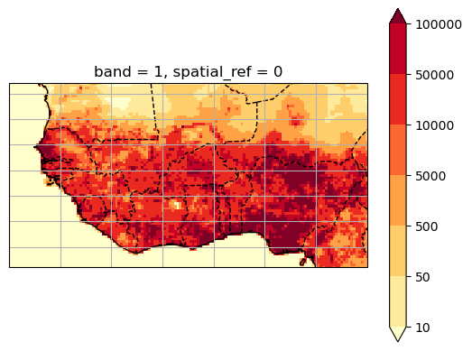
Now we have populations per ERA5 grid cell!

In a rush? Coarsen high-resolution data

In the steps above, we are conservatively regridding 1km data onto a ~25km dataset (ERA5). The regridding takes time because the algorithm is careful in preserving the population density. To be honest, we could do a very similar job with a coarser resolution data. Let’s try that:

worldpop_5km = worldpop.coarsen(longitude=5, latitude=5, boundary='trim').sum()  # We are counting population here, so sum() it is
worldpop_5km.shape

(432, 840)

This is much more manageable. Let’s regrid this:

# Calculate pop density
dx_5km = np.deg2rad(worldpop_5km.longitude[1] - worldpop_5km.longitude[0]) 
area_5km = worldpop_5km * 0 + earth_radius_km**2 * dx_5km**2 * np.cos(np.deg2rad(worldpop_5km.latitude))
density_5km = worldpop_5km / area_5km

# Regrid (takes much less time)
regridder = xe.Regridder(density_5km, annual_prcp, method='conservative')
density_5km_on_era = regridder(density_5km)
    
# And convert the population density back to population totals:
dx_era = np.deg2rad(ds.longitude[1] - ds.longitude[0]) 
era_area_km = annual_prcp * 0 + earth_radius_km**2 * dx_era**2 * np.cos(np.deg2rad(ds.latitude))
worldpop_5km_on_era5 = density_5km_on_era * era_area_km

Check the difference to the “exact” solution:

(worldpop_5km_on_era5 - worldpop_on_era5).plot(cmap='RdBu', vmin=-1e4, vmax=1e4);

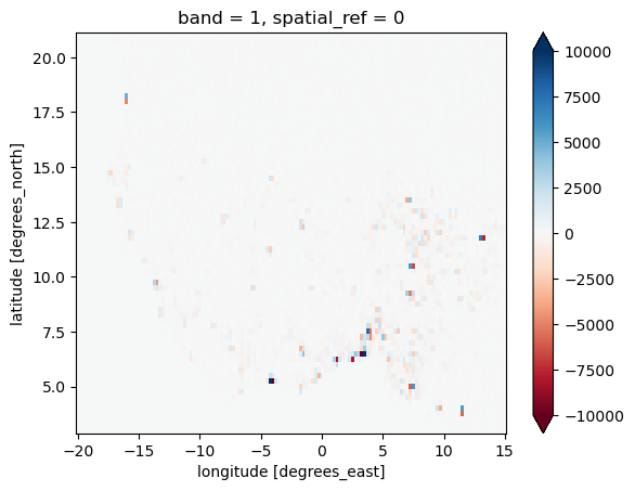
There are some small differences but they are not really relevant in context:

worldpop_5km_on_era5.sum().item(), worldpop_on_era5.sum().item()

(445909206.78588235, 445909198.7850304)