Lesson 02: geospatial datasets

In this lesson we will use a typical use case in glacier research as an opportunity to learn about geospatial joins: a very common operation in climate risk analysis, to align datasets with each other.

The main question we are trying to address is: how do we know which of the > 200’000 glaciers worldwide are located in the Rhone basin? And in the Indus basin? And in the other basins?

This question is similar to asking: which cities were affected by the drought, if I know the location of cities and the extent of the drought? And many similar questions.

Let’s start by importing the packages. We have a new package this week!

This workshop and the next require the installation of new python packages. This needs to be done once on the machine you are running this notebook. Find the instructions below.

Installing additional packages in an existing environmnent is easy:

1. Start by opening a prompt and activating the qcr environment as usual: conda activate qcr

2. Now, install the requested packages. Let’s install a few at a time: type mamba install --channel conda-forge cftime geopandas rioxarray (or, if mamba is not available, conda install --channel conda-forge cftime geopandas rioxarray). Answer yes to the questions.

3. That’s it! you can start jupyter-lab as usual.

After having completed the steps above, this should run without error:

import numpy as np
import matplotlib.pyplot as plt
import xarray as xr
import pandas as pd
from cartopy import crs as ccrs
import geopandas as gpd  # This is new!
import shapely.geometry as shpg  # This is new as well

We introduce two new packages:

• GeoPandas extends Pandas to handle spatial data, making it easier to work with geographic datasets such as river basins, and much, much more.

• Shapely provides geometric objects and operations, which geopandas uses under the hood to manipulate spatial features. We’ll cross that bridge when it comes.

Glacier locations and other global statistics

Head to the data download page and download the two files:

• glacier_basins.zip: I put this file in a new glaciers folder I created in the data folder, and extracted it (the zip extraction is important!)

• rgi60_stats.csv: I also put this file in the glaciers folder

The rgi60_stats.csv is a csv file - we know how to deal with these files now!

rgi_df = pd.read_csv('../data/glaciers/rgi60_stats.csv', index_col=0)

Explore the dataframe, its structure, length, etc.

# Your answer here

This table was generated based on the Randolph Glacier Inventory version 6.

Here are a few explanations for the most relevant columns:

• RGIId: The unique identifier for each glacier in the Randolph Glacier Inventory (RGI).

• BgnDate: The date of the satellite image used to delineate the glacier, in YYYYMMDD format.

• CenLon, CenLat: The central longitude and latitude of the glacier, representing its approximate centroid.

• O1Region, O2Region: The primary and secondary region codes according to the RGI classification. These help categorize glaciers by geographic location.

• Area: The glacier’s total surface area in square kilometers (km²).

• Zmin, Zmax, Zmed: The minimum, maximum, and median elevation of the glacier in meters above sea level (m a.s.l.).

• Slope: The average surface slope of the glacier, measured in degrees.

• Aspect: The dominant aspect (orientation) of the glacier, measured in degrees (0° = North, 90° = East, 180° = South, 270° = West).

• Name: The given name of the glacier, if available. Many glaciers remain unnamed and are recorded as NaN.

This dataset provides a static snapshot of glaciers at the time of their delineation, meaning it does not track their changes over time. The RGI’s primary goal is to provide glacier outlines - to reduce the dataset I scrapped the outlines out of the file and only provide the outlines attributes.

Q: Here are a few questions to get you started:

• how many glaciers are there in the RGI?

• what is their total area?

• what is the maximum glacier elevation?

• can you plot a histogram of the Aspect of the glaciers? What is the dominant direction of glaciers? Was it predictable?

• optional: select all glaciers in the northern hemisphere, and repeat the histogram

• optional: now group the glaciers per O1Region category (hint: groupby()), and compute the total area per RGI region.

# Your answer here

The RGI glaciers are organised in main regions as shown on the map below. Many publications will refer to these regions, but you may notice that they are not very useful from an adaptation standpoint. Communities and water resource managers will be more likely to be interested in river basins. It’s the motivation behind this lesson.

There is a lot more we could explore with this dataset, but we have to get going with more pressing matters.

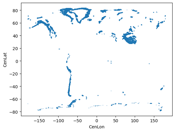
For our main goal (attributing glaciers to a given basin), the CenLon and CenLat columns might be useful. I can start by plotting the glacier locations on a scatter plot, but this is not really “geospatial” yet:

rgi_df.plot.scatter(x='CenLon', y='CenLat', s=0.1);

We’ll get back to glacier locations once we are aquainted with the river basins file.

River basins shapefile

Let’s open the second dataset you downloaded. You should have a glacier_basins folder containing five files. In a way, these are all parts of the same dataset, which is referenced by the main file: glacier_basins.shp.

A shapefile is a widely used format for storing vector data in Geographic Information Systems (GIS). Shapefiles store vector data, which represents geographic features using Points (e.g., glacier centroids), Lines (e.g., river networks), Polygons (e.g., glacier outlines and basins).

Unlike raster data (grids of pixels), vector data allows for precise geographic representation and rich attribute information, and it is structured very differently.

You can now load the glacier_basins.shp file using GeoPandas to explore its content:

gdf = gpd.read_file('../data/glaciers/glacier_basins/glacier_basins.shp')  

gdf is called a “geodataframe”. You’ll find it very convenient! It ressembles a very standard pandas dataframe, except for one column (geometry):

gdf

	MRBID	RIVER_BASI	CONTINENT	OCEAN	SEA	AREA_CALC	Shape_Leng	Shape_Area	RGI_AREA	geometry
0	2103	INDIGIRKA	Asia	Arctic Ocean	East Siberian Sea	341234.0	85.604051	70.212499	171.941	POLYGON ((151.725 70.975, 151.725 70.97083, 15...
1	2108	OB	Asia	Arctic Ocean	Kara Sea	3040606.1	168.355250	448.342075	763.493	POLYGON ((91.75 57.70417, 91.74542 57.70299, 9...
2	2302	BRAHMAPUTRA	Asia	Indian Ocean	Bay of Bengal	540782.5	66.054440	49.686611	10528.496	POLYGON ((97.76667 28.77083, 97.76335 28.77168...
3	2306	GANGES	Asia	Indian Ocean	Bay of Bengal	1006558.6	122.349983	90.946880	7906.081	MULTIPOLYGON (((88.02555 21.5715, 88.02361 21....
4	2309	INDUS	Asia	Indian Ocean	Arabian Sea	865012.6	81.286291	82.852275	27206.546	MULTIPOLYGON (((67.44167 23.97006, 67.44028 23...
...	...	...	...	...	...	...	...	...	...	...
70	6241	PO	Europe	Atlantic Ocean	Adriatic Sea	73289.5	21.576098	8.425867	313.417	POLYGON ((9.68333 46.425, 9.68418 46.42168, 9....
71	6242	RHINE	Europe	Atlantic Ocean	North Sea	163122.3	48.247612	20.200160	336.922	POLYGON ((4.45638 52.14527, 4.46175 52.1411, 4...
72	6243	RHONE	Europe	Atlantic Ocean	Mediterranean Sea	96637.6	28.004916	11.197342	917.302	POLYGON ((6.84167 47.82083, 6.84167 47.81667, ...
73	6254	THJORSA	Europe	Atlantic Ocean	North Atlantic	8277.8	9.270847	1.545336	972.419	POLYGON ((-17.5 64.625, -17.50035 64.60591, -1...
74	6255	TORNEALVEN (also TORNIONJOKI, also TORNIONVAYLA)	Europe	Atlantic Ocean	Baltic Sea	40545.2	28.919025	8.685652	34.257	POLYGON ((23.69167 68.84167, 23.70214 68.84102...

75 rows × 10 columns

Operations that work on a dataframe also work on a geodataframe. For example, we can count the number of basins per continent:

gdf.groupby('CONTINENT').count()[['geometry']]

	geometry
CONTINENT
Asia	19
Europe	15
North America, Central America and the Caribbean	16
South America	24
South-West Pacific	1

Q: Here are a few questions to get you started:

• how many basins are there in the file?

• what is their total area? (hint: AREA_CALC, in km2)

• can you print the list of all their names?

# Your answer here

Note that this dataset contains a subset of all of the word basins. These are all of the world’s large river basins (> 3000 km²) with considerable glacier cover (> 30 km²). The original dataset (not cropped for glaciers) can be found at the Global Runoff Data Centre - Major River Basins.

Using standard pandas methods, we can also compute the total area of glaciers contained in these basins:

gdf['RGI_AREA'].sum()

np.float64(162804.435)

Note: This is much less than the total area of glaciers worldwide you compute above, because many glaciers in the polar regions do not have an assigned basin.

We can also compute a useful new statistic: the % of the basin which is covered by glaciers:

gdf['glacier_cover'] = (gdf['RGI_AREA'] / gdf['AREA_CALC']) * 100

E: plot a histogram of the glacier_cover data. What is the median glacier cover? And what is the basin with the highest percentage of glacier cover?

# Your answer here

Plotting with geopandas

So far, this all looked very similar to “standard” pandas. So, what’s the deal with Geopandas? It offers many services, but the main ones are:

1. Plotting vector data from the geometry column (this section)

2. Geospatial operations on the geometry column (next section)

Let’s ask for the simplest plot of all:

gdf.plot(ec='k');

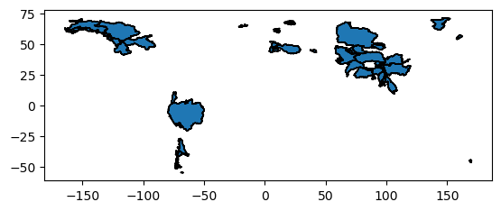
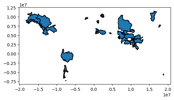
The basin shapes are provided in the WGS84 (standard lon-lat) projection. Geopandas also comes with handy tools to convert this to any other projection if needed:

gdf.to_crs(epsg="3857").plot(ec='k');

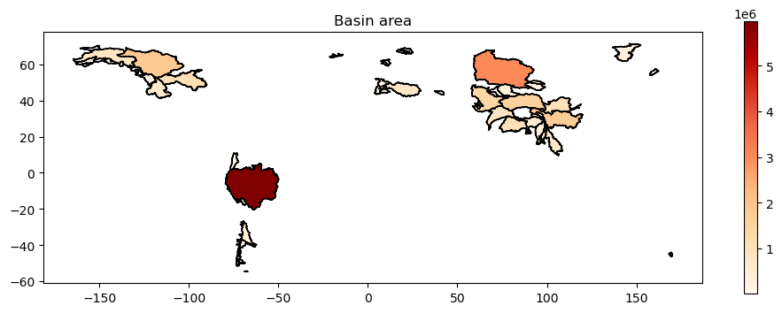
Geopandas also comes with a lot of handy ways to plot the data, but we’ll learn only one today: assigning colors to attributes of the geometries. Here coloring by basin area:

f, ax = plt.subplots(figsize=(12, 4))
gdf.plot(ax=ax, column="AREA_CALC", cmap="OrRd", ec='k', legend=True);
plt.title('Basin area');

Exercise: now plot the basins again but the color indicating glacier area, not basin area. Then continue with the percentage glacier area per basin (glacier_cover).

# Your answer here

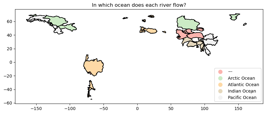
One can also plot categorical data! See by yourself:

f, ax = plt.subplots(figsize=(12, 4))
gdf.plot(ax=ax, column="OCEAN", categorical=True, cmap="Pastel1", ec='k', 
         legend=True, legend_kwds={"loc": "lower right"});
plt.title('In which ocean does each river flow?'); 

And, finally, one can plot geopandas dataframe on any map projection with cartopy, very much like raster data in the first two workshops:

# Create figure with custom figsize and projection
fig, ax = plt.subplots(figsize=(12, 4), subplot_kw={"projection": ccrs.Robinson()})
gdf.plot(ax=ax, column="OCEAN", categorical=True, cmap="Pastel1", ec='k', 
         legend=True, legend_kwds={"loc": "lower right"},
         transform=ccrs.PlateCarree());
plt.title('In which ocean does each river flow?'); 
ax.coastlines(color='grey');  # Add coastlines
ax.set_global();  # Global plot

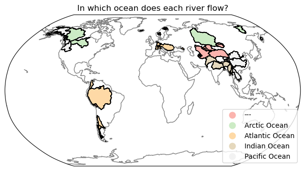
In the plot above, what does the --- basin represent? Is there a name for such basins?

# Your answer here

Finding out in which basin each glacier belongs

So far, we have a dataset of glaciers (rgi_df) with their geographic coordinates (CenLon, CenLat), but no spatial information about which river basin they belong to. On the other hand, we have a GeoDataFrame (gdf) that contains the river basin boundaries as polygons.

To assign each glacier to a basin, we will:

1. Convert glacier locations into geometries: We will transform CenLon and CenLat into Shapely Point objects, creating a GeoDataFrame from rgi_df.

2. Use a spatial join: We will use geopandas.sjoin() to determine which basin each glacier falls into.

3. Store the basin information: The result will be a new column in rgi_df that tells us which basin each glacier belongs to.

This is a common GIS task in climate impact studies, as linking a dataset to another is a very important step for most impact or vulnerability assessment. Let’s do it!

# Step 1: Convert RGI dataframe into a GeoDataFrame with Point geometries
rgi_gdf = gpd.GeoDataFrame(
    rgi_df,
    geometry=gpd.points_from_xy(rgi_df['CenLon'], rgi_df['CenLat']),
    crs="EPSG:4326"  # This is WGS84 - the same coordinate reference system as the basins
)

# Step 2: Perform a spatial join (each glacier gets assigned a basin)
rgi_gdf = gpd.sjoin(rgi_gdf, gdf, how="left", predicate="within")

# Step 3: Store results back in the original dataframe
rgi_df['MRBID'] = rgi_gdf['MRBID']

That’s it! Let’s see what we’ve got:

rgi_df

	BgnDate	CenLon	CenLat	O1Region	O2Region	Area	Zmin	Zmax	Zmed	Slope	Aspect	Name	MRBID
RGIId
RGI60-01.00001	20090703	-146.8230	63.6890	1	2	0.360	1936	2725	2385	42.0	346	NaN	4435.0
RGI60-01.00002	20090703	-146.6680	63.4040	1	2	0.558	1713	2144	2005	16.0	162	NaN	4430.0
RGI60-01.00003	20090703	-146.0800	63.3760	1	2	1.685	1609	2182	1868	18.0	175	NaN	4435.0
RGI60-01.00004	20090703	-146.1200	63.3810	1	2	3.681	1273	2317	1944	19.0	195	NaN	4435.0
RGI60-01.00005	20090703	-147.0570	63.5510	1	2	2.573	1494	2317	1914	16.0	181	NaN	4430.0
...	...	...	...	...	...	...	...	...	...	...	...	...	...
RGI60-19.02748	20020502	-37.7325	-53.9860	19	3	0.042	310	510	-999	29.9	315	NaN	NaN
RGI60-19.02749	20030207	-36.1361	-54.8310	19	3	0.567	330	830	-999	23.6	200	NaN	NaN
RGI60-19.02750	20030207	-37.3018	-54.1884	19	3	4.118	10	1110	-999	16.8	308	NaN	NaN
RGI60-19.02751	19870101	-90.4266	-68.8656	19	1	0.011	170	270	-999	0.4	122	AQ6C10200013	NaN
RGI60-19.02752	19660301	37.7140	-46.8972	19	4	0.528	970	1170	-999	9.6	35	ZA6C40100001 Ice Plateau	NaN

215547 rows × 13 columns

We’ve added a new column (MRBID) which assigns a glacier to each basin. Or does it?

Q: answer the following questions:

• how many glaciers are assigned to the basin 6243 (Rhone)? Does it match what you computed in lesson 01?

• what is the area of all glaciers in the Rhone?

• how many glaciers are not attributed to any basin? What is the area of all glaciers with and without a basin?

• grouping by basin id: what is the basin with the highest avereage median elevation? and the lowest?

# Your answer here

Conclusions & next steps: unlocking more detailed spatial analyses

In this lesson, we expanded our geospatial toolkit to move beyond predefined large basins. Instead of relying on fixed datasets, you now have the ability to:

• Select and analyze specific hydrological basins based on your own criteria.

• Use geospatial tools to link climate impacts (such as glacier runoff, precipitation, or extreme events) to specific catchments.

• Define study areas more flexibly, allowing for more detailed and localized analysis.

This unlocks new possibilities for climate impact assessments. While large-scale basins are useful for broad regional trends, many of the most important hydrological changes occur in smaller catchments where local conditions—such as runoff sources, land cover, or topography—play a major role.

With these tools, you can now:

• Study individual tributaries and sub-basins, rather than relying only on large drainage areas.

• Analyze regions where small-scale hydrological changes matter, such as flood-prone areas, water-stressed basins, or high-elevation catchments.

• Investigate extreme events, like glacial lake outburst floods, heavy precipitation events, or seasonal water availability shifts in a spatially explicit way.

As you move forward, think about how the spatial scale of your analysis affects your conclusions—some insights may be lost in large-scale averages but become clear when looking at localized basin-scale changes.