Correction of the exam 2023#
There were 5 exam questions:
2 multiple choice
1 short programming exercise
2 longer notebooks
Multiple choice: Environments#
Which following statements about python packages and conda environments are true? Careful: wrongly ticked answers will give negative points!
When a python package is installed in the base conda environment, it is also installed per default in any other conda environment.
Answer: Wrong. Lecture notes on the topic: Recommended: create an environment called “inpro”
“mamba install” is very similar to “conda install”, but is usually faster.
Answer: Correct. Lecture notes on the topic: Context: conda environments. Google also knows the answer.
There are different kinds of python interpreters. “ipython” is one one of them.
Answer: Correct. Google knows the answer.
numpy is part of the python standard library.
Answer: Wrong. Google knows the answer.
Multiple choice: Indexing#
Which of the affirmations about the code snippet below are true?
import numpy as np

a = np.arange(12).reshape((3, 4))
b = a * 2
nz = np.nonzero(a > 8)
b[nz] = a[nz]
Wrong answers are penalized! In case of doubt you may choose not to answer.
This code produces an array b which doubles the values in a, except where the values are strictly larger than 8. In this case, the values are not doubled.
Answer: correct. Running the code might have been the best strategy to answer this.
The same result can be obtained using boolean indexing.
Answer: Correct. This would be the code:
import numpy as np

a = np.arange(12).reshape((3, 4))
b = a * 2
larger_than_8 = a > 8
b[larger_than_8] = a[larger_than_8]
Lecture notes on the topic: Selecting parts of an array with boolean indexing.
The code uses boolean indexing.
Answer: Wrong. It uses positional indexing, by asking first where (at which position) are the elements which are larger than 8, and then using these positions to index a and b: therefore, positional indexing. Lecture notes on the topic: Selecting parts of an array with positional indexing.
The code uses positional indexing.
Answer: Correct. It uses positional indexing, by asking first where (at which position) are the elements which are larger than 8, and then using these positions to index a and b: therefore, positional indexing. Lecture notes on the topic: Selecting parts of an array with positional indexing.
Coding: Taylor function#
Write a function called taylor_sin which computes the Taylor approximation of the sinus function:
With ! denotating the number’s factorial. The inputs n and x should be given as argument to the function. Quantify the uncertainty of the approximation for x = π / 2 and n=5.
Answer:
import math

def taylor_sin(x, n):
    output = 0
    for i in range(n+1):
        output += (-1)**i * x**(2*i+1) / math.factorial(2*i+1)
    return output

x = math.pi / 2


true_value = math.sin(x)

n = 5
print(f'Error for x = π / 2 and n={n}: {taylor_sin(x, n) - true_value}')
Error for x = π / 2 and n=5: -5.625894905492146e-08
Other values of n:
for n in [1, 3, 5, 7]:
    print(f'Error for x = π / 2 and n={n}: {taylor_sin(x, n) - true_value}')
Error for x = π / 2 and n=1: -0.07516777071134961
Error for x = π / 2 and n=3: -0.00015689860050127624
Error for x = π / 2 and n=5: -5.625894905492146e-08
Error for x = π / 2 and n=7: -6.023181953196399e-12
Notebook: Greenland#
Here is a link to a .csv file to download:
https://cluster.klima.uni-bremen.de/~fmaussion/teaching/inpro/greenland.csv
It contains data from an automatic weather station at the North of the Greenland ice-sheet. It contains the measured incoming (“down”) and outgoing (“up”) shorwtave radiation at the station.
Your task is to return a Jupyter Notebook (upload button) which does the following:
import pandas as pd
import numpy as np
import matplotlib.pyplot as plt
1. Read the csv file using pandas, and make sure the index of the DataFrame has the datatype DatetimeIndex.
df = pd.read_csv('https://cluster.klima.uni-bremen.de/~fmaussion/teaching/inpro/greenland.csv', index_col=0, parse_dates=True)
df.index
DatetimeIndex(['2010-01-01 00:00:00', '2010-01-01 01:00:00',
               '2010-01-01 02:00:00', '2010-01-01 03:00:00',
               '2010-01-01 04:00:00', '2010-01-01 05:00:00',
               '2010-01-01 06:00:00', '2010-01-01 07:00:00',
               '2010-01-01 08:00:00', '2010-01-01 09:00:00',
               ...
               '2016-12-31 14:00:00', '2016-12-31 15:00:00',
               '2016-12-31 16:00:00', '2016-12-31 17:00:00',
               '2016-12-31 18:00:00', '2016-12-31 19:00:00',
               '2016-12-31 20:00:00', '2016-12-31 21:00:00',
               '2016-12-31 22:00:00', '2016-12-31 23:00:00'],
              dtype='datetime64[ns]', name='datetime', length=61368, freq=None)
2. For both data columns, replace missing values with NaN (missing values can be found easily)
df = df.replace(-999., np.nan)
3. Select data from the years 2010 to 2015 only (i.e. discard the incomplete year 2016). From now on, we only analyze data from 2010 to 2015.
df = df.loc['2010':'2015']
4. Compute the average albedo at this location, which is computed as: \(\sum SW_{up} / \sum SW_{down}\) over the entire time period from 2010 to 2015.
albedo = df['ShortwaveRadiationUp_Cor(W/m2)'].sum() / df['ShortwaveRadiationDown_Cor(W/m2)'].sum()
albedo
0.768098221597999
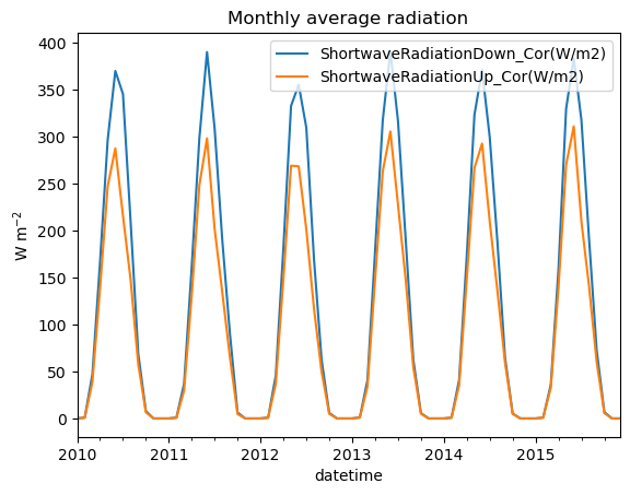
5. Compute the monthly average radiation from the data, and plot it on a line plot (see example below). Tip: if you don’t manage this question, you can still do the rest of the exercise independently.
df.resample('MS').mean().plot();
plt.ylabel('W m$^{-2}$');
plt.title('Monthly average radiation');
6. Compute the daily cycle of radiation (average hourly radiation) for the month of June. I expect a DataFrame with index of type integer, with values from 0 to 23.
dfs = df.loc[df.index.month == 6]
dfs = dfs.groupby(dfs.index.hour).mean()
dfs.index
Index([ 0,  1,  2,  3,  4,  5,  6,  7,  8,  9, 10, 11, 12, 13, 14, 15, 16, 17,
       18, 19, 20, 21, 22, 23],
      dtype='int32', name='datetime')
7. Using the hourly average data from question 6: at what time of day in the incoming radiation largest? What is its value?
dfs['ShortwaveRadiationDown_Cor(W/m2)'].max()
577.3088888888889
dfs['ShortwaveRadiationDown_Cor(W/m2)'].idxmax()
14
or:
dfs['ShortwaveRadiationDown_Cor(W/m2)'].loc[dfs['ShortwaveRadiationDown_Cor(W/m2)'] == dfs['ShortwaveRadiationDown_Cor(W/m2)'].max()]
datetime
14    577.308889
Name: ShortwaveRadiationDown_Cor(W/m2), dtype: float64
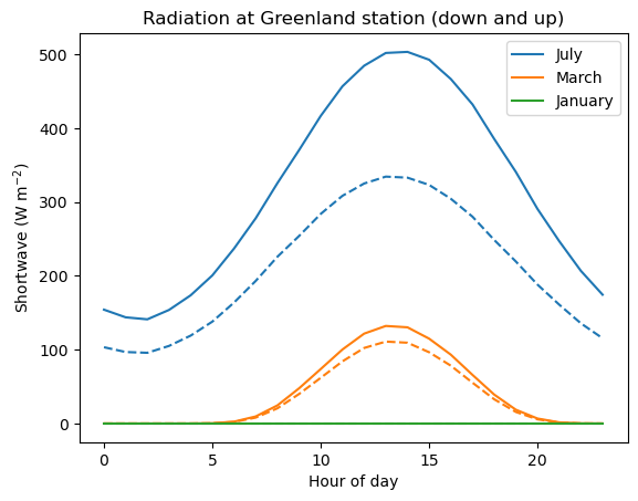
8. Plot the daily cycle of hourly incoming radiation in January, March and July as line plot. Tip: the x-axis of the plot should show the hour of the day, from 0 to 23. Add the outgoing radiation as a dashed line (see example plot below).
dfs = df.loc[df.index.month == 7]
dfs = dfs.groupby(dfs.index.hour).mean()
dfs['ShortwaveRadiationDown_Cor(W/m2)'].plot(label='July', color='C0');
dfs['ShortwaveRadiationUp_Cor(W/m2)'].plot(label='', linestyle='--', color='C0');


dfs = df.loc[df.index.month == 3]
dfs = dfs.groupby(dfs.index.hour).mean()
dfs['ShortwaveRadiationDown_Cor(W/m2)'].plot(label='March', color='C1');
dfs['ShortwaveRadiationUp_Cor(W/m2)'].plot(label='', linestyle='--', color='C1');

dfs = df.loc[df.index.month == 1]
dfs = dfs.groupby(dfs.index.hour).mean()
dfs['ShortwaveRadiationDown_Cor(W/m2)'].plot(label='January', color='C2');
dfs['ShortwaveRadiationUp_Cor(W/m2)'].plot(label='', linestyle='--', color='C2');

plt.legend(); plt.ylabel('Shortwave (W m$^{-2}$)'); plt.xlabel('Hour of day'); plt.title('Radiation at Greenland station (down and up)');
Notebook: Peru#
Here is a code snippet which loads 2D data from the web:
from urllib.request import Request, urlopen
from io import BytesIO
import numpy as np

# Parse the given url
url = 'https://cluster.klima.uni-bremen.de/~fmaussion/teaching/inpro/chirps_peru_avg.npz'
req = urlopen(Request(url)).read()
with np.load(BytesIO(req)) as data:
    annual_prcp = data['annual_prcp']
    lon = data['lon']
    lat = data['lat']
Copy this code snippet and paste it in an empty notebook. Execute the code.
annual_prcp is a numpy array of shape (lat, lon) and represents the average annual precipitation (unit mm/d) over the country of Peru.
Upload a Jupyter Notebook (upload button) which addresses the following tasks. Tip: many of the tasks can be done independently from the other ones! Pick the ones you know how to do quickly.
1. Compute annual_prcp_myr, the average annual precipitation in units meter per year (m yr-1). For this you can assume that a year has 365.25 days on average.
annual_prcp_myr = annual_prcp / 1000 * 365.25
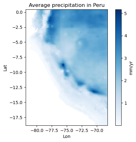
2. Plot the 2D array annual_prcp_myr with the blues colormap. Add a colorbar and ticks and axis labels (Lon, Lat). Tip: if you want your map to not be squeezed, you may have to use ax.set_aspect(‘equal’) after you plotted the data.
f, ax = plt.subplots()
im = ax.pcolormesh(lon, lat, annual_prcp_myr, shading='nearest', cmap='Blues');
ax.set_aspect('equal');
f.colorbar(im, label='mm/yr'); ax.set_xlabel('Lon'); ax.set_ylabel('Lat'); ax.set_title('Average precipitation in Peru');
3. Count the number of pixels in annual_prcp_myr which have a precipitation value over 5 m yr-1.
(annual_prcp_myr > 5).sum()
6
4. Create the array annual_prcp_myr_subset, which is a subset of the annual_prcp_myr array selected between the indices 217 and 316 in latitude, and the indices 37 and 176 in longitude. The resulting 2D array should be of shape (99, 139).
annual_prcp_myr_subset = annual_prcp_myr[217:316, 37:176]
annual_prcp_myr_subset.shape
(99, 139)
5. Now create the arrays lon_subset and lat_subset, which are the corresponding coordinates selected over the same indices. lon_subset should have the shape (139,) and lat_subset should have the shape (99,).
lon_subset = lon[37:176]
lon_subset.shape
(139,)
lat_subset = lat[217:316]
lat_subset.shape
(99,)
6. Now average annual_prcp_myr_subset over the latitudes to create an array of shape (139,) named annual_prcp_myr_subset_lat.
annual_prcp_myr_subset_lat = annual_prcp_myr_subset.mean(axis=0)
annual_prcp_myr_subset_lat.shape
(139,)
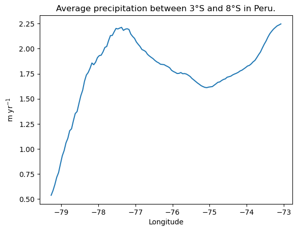
7. Plot annual_prcp_myr_subset_lat as a line plot as the example plot below.
plt.plot(lon_subset, annual_prcp_myr_subset_lat);
plt.title('Average precipitation between 3°S and 8°S in Peru.')
plt.xlabel('Longitude'); plt.ylabel('m yr$^{-1}$');
8. Using a numpy function you learnt during the lecture, find out why I chose the indices 217 and 316 to select data for latitudes between -3° and -8°.
p = np.nonzero((lat < -3) & (lat >-8))[0]
p
array([217, 218, 219, 220, 221, 222, 223, 224, 225, 226, 227, 228, 229,
       230, 231, 232, 233, 234, 235, 236, 237, 238, 239, 240, 241, 242,
       243, 244, 245, 246, 247, 248, 249, 250, 251, 252, 253, 254, 255,
       256, 257, 258, 259, 260, 261, 262, 263, 264, 265, 266, 267, 268,
       269, 270, 271, 272, 273, 274, 275, 276, 277, 278, 279, 280, 281,
       282, 283, 284, 285, 286, 287, 288, 289, 290, 291, 292, 293, 294,
       295, 296, 297, 298, 299, 300, 301, 302, 303, 304, 305, 306, 307,
       308, 309, 310, 311, 312, 313, 314, 315, 316])
p.min(), p.max()
(217, 316)