Scientific python#
You have learned so many things in this lecture, I hope that you are proud of yourself! Starting with no programming experience at all, you are now able to use a python interpreter to open various text files, analyze data, and make plots. This is great, and gives you enough background to tackle more difficult problems.
In the course of your studies, you will meet other new challenges frequently. I hope that the elements you’ve learned in this class so far will help you to overcome the first obstacles, but I’m also certain that you will need a fair amount of googling and learning to get things done.
Therefore, this final lesson is not really a “lesson”, it’s a collection of links and suggestions for some very common tasks in the geosciences. You might come back to it later in your studies.
The scientific python stack#
Unlike Matlab, the set of Python tools used by scientists does not come from one single source. It is the result of a non-coordinated, chaotic but creative development process originating from a community of volunteers and professionals.
The set of python scientific packages is sometimes referred to as the “scientific python ecosystem”. I didn’t find an official explanation for this name, but I guess that it has something to do with the fact that many packages rely on the others to build new features on top of them, like a natural ecosystem.
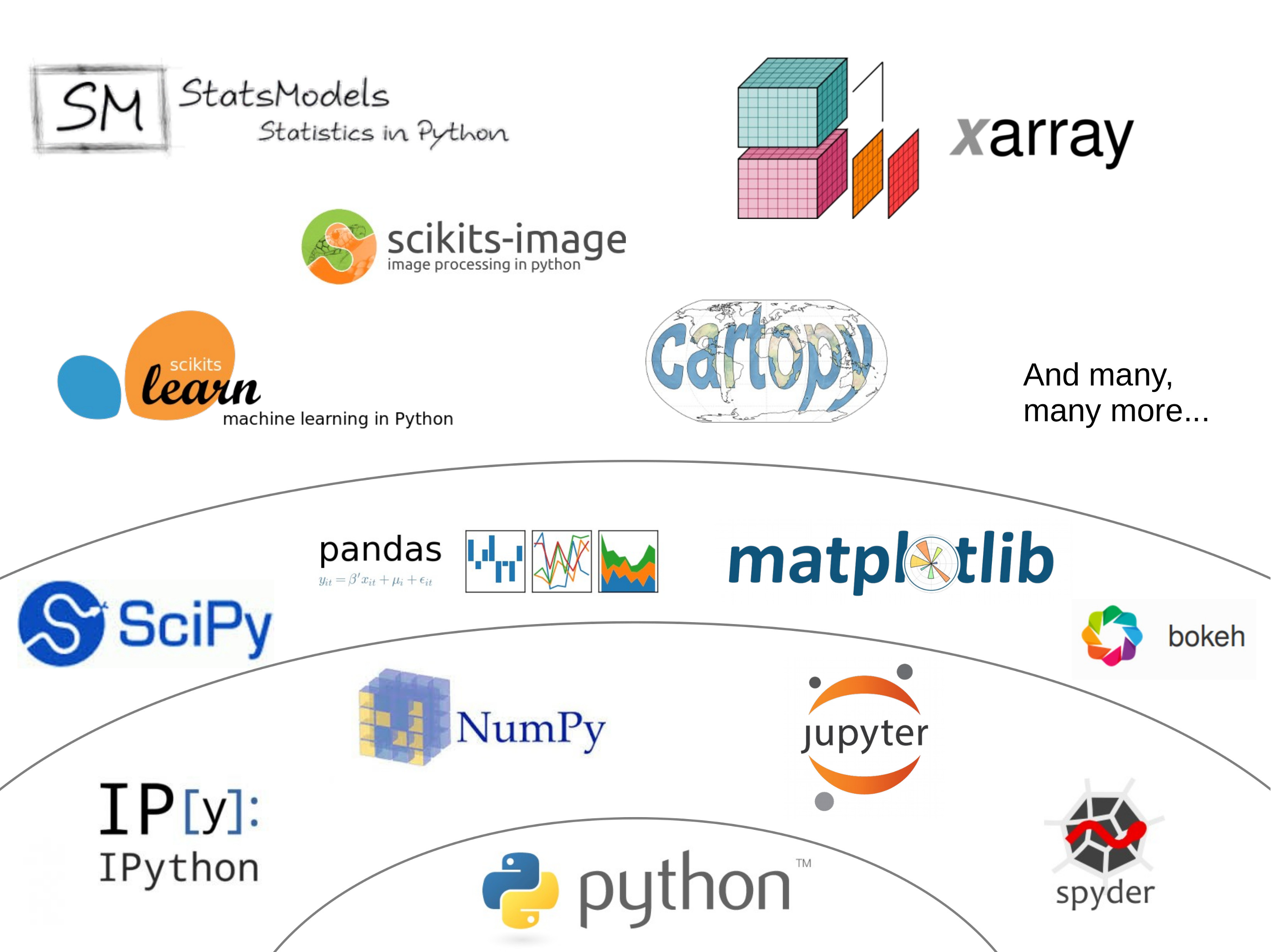
Jake Vanderplas made a great graphic in a 2015 presentation (the video of the presentation is also available here if you are interested), and I took the liberty to adapt it a little bit:
The core packages#
You already know the most important ones:
ipython and jupyter add interactivity (and much more) to the python interpreter.
numpy provides the N-dimensional arrays necessary to do fast computations.
scipy is the scientist’s toolbox. It is a very large package and covers many aspects of the scientific workflow, organized in submodules, all dedicated to a specific aspect of data processing. For example: scipy.integrate, scipy.optimize, or scipy.linalg.
matplotlib is the traditional package to make graphics in python,
Essential numpy “extensions”#
There are two packages which I consider essential when it comes to data processing.
pandas#
pandas provides data structures designed to make working with labeled data both easy and intuitive (documentation, code repository). You already learned the basics of it in this class. I recommend to use pandas whenever you are analyzing tabular (column) data.
When not to use pandas though? In a few cases:
when the data is not columnar, but multi-dimensional. For this, use xarray (see below).
when performance matters (e.g. numerical simulations). In this case, stay with numpy arrays and use pandas only after the computations are done.
xarray#
xarray is very similar to pandas, but for N-dimensional arrays (documentation, code repository).
xarray is a fundamental tool in geosciences, and you will learn about it in the climate lectures. It will be your tool of choice when opening netcdf files and plot maps in combination with cartopy. More about this soon in the climate lectures. But in the meantime, you can visit the xarray recipe in the lecture notes.
Domain specific packages#
There are so many of them! I can’t list them all, but here are a few that you will probably come across in your studies or career:
Geosciences/Meteorology:
MetPy: the meteorology toolbox
Cartopy: maps and map projections
xESMF: Universal Regridder for Geospatial Data
xgcm: General Circulation Model Postprocessing with xarray
GeoPandas: Pandas for vector data
Rasterio: geospatial raster data I/O
Statistics/Machine Learning:
Statsmodels: statistic toolbox for models and tests
Seaborn: statistical data visualization
Scikit-learn: machine learning tools
TensorFlow: Google’s brain
PyTorch: Facebook’s brain
Miscellaneous:
imageio: read image files
Scikit-image: image processing
Bokeh: interactive plots
Dask: parallel computing
…