Assignment 07#
Due date: 17.05.2023
This week’s assignment has to be returned in the form a jupyter notebook.
Don’t forget the instructions!
01 - Linear equations#
Using numpy alone, solve the following system of linear equations:
To solve it, remember that in matrix notation, \(A x = y\) can be refactored to \(x = A^{-1} y\), if \(A\) is an invertible matrix, and \(x\) and \(y\) are vectors. Use numpy to invert the matrix \(A\) and solve for \(x\).
# Your answer here
02 - A simple Earth Energy Balance model#
Let’s imagine a simple 1-layer model of our planetary climate system. We will try to compute its energy balance.
In space, the only source of incoming energy is that of the sun. The sun energy per unit area (\(W m^{-2}\)) reaching earth is the solar constant \(S_0\): its value is approximately 1362 \(W m^{-2}\). This energy is distributed from a circle to the sphere (cf. climate lecture), which implies that only a quarter of it is available on average over the globe. Part of this energy is reflected directly to space (mostly by clouds and ice) according to the planetary albedo \(\alpha = 0.32\).
Therefore, the total energy entering the climate system (the Absorbed Shortwave Radiation or ASR) is:
At human time scales, \(S_0\) is a constant, while \(\alpha\) may change with time.
Define a function asr which takes one optional keyword argument alpha (which defaults to 0.3) and returns the ASR (\(W m^{-2}\)):
def asr(alpha=0.3):
    """Absorbed Solar Radiation (W m-2).

    Parameters
    ----------
    alpha : float, optional
        the planetary albedo

    Returns
    -------
    the asr (float)

    Examples
    --------
    >>> print(f'{asr():.2f}')
    238.35
    >>> print(f'{asr(alpha=0.32):.2f}')
    231.54
    """
    < your code here >
# Testing
import doctest
doctest.testmod()
TestResults(failed=0, attempted=0)
Plot the ASR as a function of albedo, for the range [0.2, 0.7]:
# Your answer here
This incoming solar energy is warming up the climate system which, in turn, emits longwave radiation. Using Stefan Boltzmann’s law, the Outgoing Longwave Radiation (OLR) is therefore:
with \(T\) the atmosphere temperature in Kelvin, \(\sigma\) the Stefan Boltzmann constant (\(5.67 \times 10^{-8}\)) and \(\tau\) the transmissivity of the atmosphere (let’s say it is 0.611 - a value I tuned to match the observed OLR).
Define a function olr which takes one positional argument t and one optional keyword argument tau (which defaults to 0.611) and which returns the OLR (\(W m^{-2}\)):
def olr(t, tau=0.611):
    """Outgoing Longwave Radiation (W m-2).

    Parameters
    ----------
    t : float
        the atmosphere temperature (K)
    tau : float, optional
        the atmosphere transmissivity (-)

    Returns
    -------
    the olr (float)

    Examples
    --------
    >>> print(f'{olr(288):.2f}')
    238.34
    >>> print(f'{olr(288, tau=0.63):.2f}')
    245.75
    """
    < your code here >
# Testing
import doctest
doctest.testmod()
TestResults(failed=0, attempted=0)
Plot the OLR as a function of temperature, for the range [270 300]. Repeat with tau=0.5 and tau=0.7 (three lines on the same plot, with a legend).
# Your answer here
Verify that with the default parameters and an atmosphere temperature of 288K, the climate system is approximately in energy balance (ASR == OLR, \(\pm 0.02 W m^{-2}\)).
# Your answer here
Humans started to emit greenhouse gases to the atmosphere. Since greenhouse gases are trapping heat, this has the consequence to reduce the transmissivity of the atmosphere.
Compute the energy imbalance of the climate system (\(\Delta E = ASR -OLR\)) if \(\tau\) is reduced to 0.59 but the temperature stays constant at 288.
# Your answer here
Written mathematically:
The change of energy over time is equal to the energy imbalance. If ASR is equal to OLR the rate of change is zero. With our emissions however we have an energy excess, which will warm um the atmosphere. The rate at which temperature increases depends on the energy imbalance and the thermal capacity of the climate system. If we suppose that:
With E the total energy of the climate system, T the temperature and C the effective heat capacity of the climate system (earth + land + ocean, assumed to be constant).
We can now write:
which is a ordinary differential equation (ODE). Let’s use forward finite differences to approximate our equation numerically:
Which we can rearrange to to solve for future temperature (\(T_{i+1}\) at time \(t + \Delta t\)) knowing present-day temperature (\(T_{i}\) ad time t):
Assuming that \(C = 4 \times 10^8 J m^2 K^{-1}\) and taking a time step of \(\Delta t = 31536000 s\) (1 year), compute \(T_1\) if \(T_0\) = 288K and the transmissivity \(\tau\) is 0.59:
C = 4.0e+08
t_0 = 288
dt = 60 * 60 * 24 * 365
# Your answer here
Now, use the strategies you learned in the lecture to write a function which computes the temperature change over time:
def temperature_change(t0, n_years, tau=0.611, alpha=0.3):
    """Temperature change scenario after change of transmissivity.

    Parameters
    ----------
    t0 : float
        the starting temperature (K)
    n_years : int
        the number of simulation years
    tau : float, optional
        the atmosphere transmissivity (-)
    alpha : float, optional
        the planetary albedo

    Returns
    -------
    (time, temperature) : ndarrays of size n_years + 1

    Examples
    --------
    >>> y, t = temperature_change(288, 2, tau=0.59)
    >>> y
    array([0, 1, 2])
    >>> print(f'{t[0]:.2f}')
    288.00
    >>> print(f'{t[1]:.2f}')
    288.65
    >>> print(f'{t[2]:.2f}')
    289.13
    """
    < your code here >
# Testing
import doctest
doctest.testmod()
TestResults(failed=0, attempted=0)
Plot the temperature change scenarios with \(\tau\) values of 0.6, 0.59, 0.58. The result should look something like this plot.
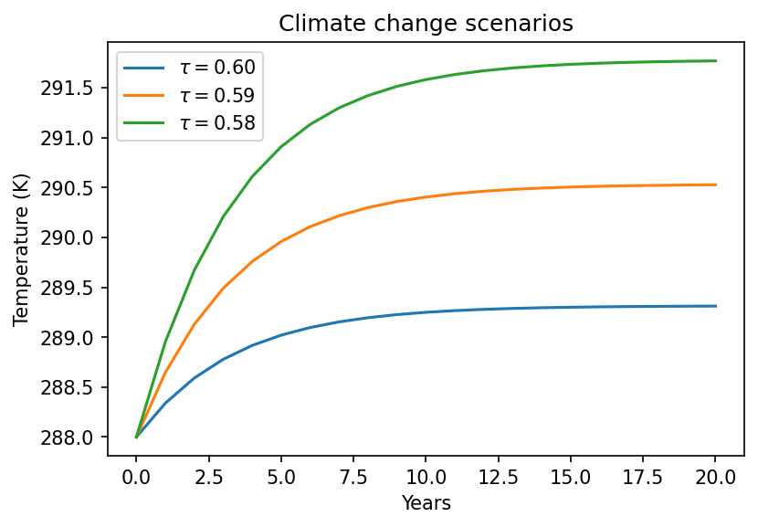
# Your answer here
Now plot the temperature change scenarios with \(\tau\) = 0.6 and starting temperatures of [288, 293].
# Your answer here
Compute the e-folding response time (in years) of this simple climate model for the scenario T=288K, \(\tau\)=0.6 (the e-folding response time is the time it takes for the system to reach 1 - 1 / e \(\approx\) 63% of the final \(\Delta T\)).
# Your answer here