Multi-dimensional numpy arrays#
You have now learned how to read and analyze 1-dimensional data with numpy (and with pandas as an additional “layer” of tools on top of the core numpy arrays).
For the final two weeks of the semester, you will learn to manipulate multi-dimensional arrays (ndarrays) which are very common in meteorology, climatology, and geosciences in general.
import numpy as np
import matplotlib.pyplot as plt
When are multidimensional arrays useful?#
For numpy, all data in any multi-dimensional array is actually stored in memory as a long 1D array (we will get back to this in the master lecture). The number of dimensions and shape of an array is actually only used to structure the data access in a certain way. But why is it useful to store data in multiple dimensions?
nD arrays as matrices#
The first time we learned about arrays as matrices was during week 07, when we learned about matrix multiplication and other linear algebra numpy functions. To use nD arrays as matrices, you have to use matrix specific operators (such as @) or functions (such at np.linalg.inv):
a = np.array([[1, 2],
              [2, 2]])
a @ np.linalg.inv(a)
array([[1., 0.],
       [0., 1.]])
Linear algebra is a very common use case for nD arrays, yet it is (by far) not the only one. I, for example, use linear algebra only sporadically in my daily work (or it is hidden behind other tools).
nD arrays as images#
Another common use case for nD arrays is to store images:
import scipy.misc

# Read a sample image from scipy
img = scipy.misc.face()

# Plot it
plt.imshow(img);
/var/folders/29/f4w56zjd1c1b_gdh_b7bjs3c0000gq/T/ipykernel_55371/3349719320.py:4: DeprecationWarning: scipy.misc.face has been deprecated in SciPy v1.10.0; and will be completely removed in SciPy v1.12.0. Dataset methods have moved into the scipy.datasets module. Use scipy.datasets.face instead.
  img = scipy.misc.face()
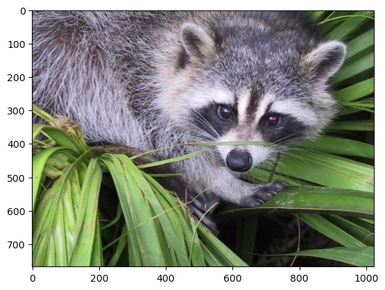
What is img? Lets find out:
img.shape, img.dtype, img.min(), img.max()
((768, 1024, 3), dtype('uint8'), 0, 255)
Here, img is a N x M x 3 array, with N the number of rows and M the number of columns. 3 is for Red, Green, Blue (RGB) channels. Here the values are mapped to the[0, 255] range, indicating the intensity of each color:
f, (ax1, ax2, ax3) = plt.subplots(1, 3, figsize=(12, 5))
ax1.imshow(img[..., 0], cmap='Reds');
ax2.imshow(img[..., 1], cmap='Greens');
ax3.imshow(img[..., 2], cmap='Blues');
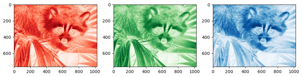
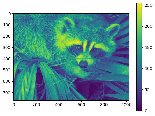
Matplotlib’s imshow understands what is meant when given 3D data with the last dimension of size 3. When given a 2D array of any type, it will map the data to a colorscale value:
data = img[..., 0]  # Select the red channel
im = plt.imshow(data);
plt.colorbar(im, orientation='vertical');
Some of the things explained above might be a bit overwhelming right now. Don’t worry! We will get back to these concepts later in this unit.
nD arrays as structured data#
Nearly all other use cases for nD arrays fall in this category. Multidimensional arrays allow to store data in the shape which is most meaningful for its analysis, display, and storage. For example:
a map of temperature of shape (Y, X) where Y are the latitudes and X the longitudes
a series of temperature maps of shape (Z, Y, X) where Z are the vertical pressure levels, Y are the latitudes and X the longitudes
a series of series of temperature maps of shape (T, Z, Y, X) where T are the time steps, Z are the vertical pressure levels, Y are the latitudes and X the longitudes
That’s the most common use case in meteorology, and the one you will have to deal with in this week’s homework. But in the course of your studies you will find many more interesting use cases, for example involving model parameters, physical quantities, time / space considerations, and more!
Working with nD arrays#
Copyright notice: parts of these examples are taken from the numpy tutorial for beginners.
Multidimensional arrays are not different from 1 dimensional arrays. In fact, it is rather the 1 dimensional array which is a special case of the multidimensional one. All methods which work on 1D arrays also apply to nD arrays.
Let’s create a 2D array:
data = np.array([[1, 2], [3, 4], [5, 6]])
data
array([[1, 2],
       [3, 4],
       [5, 6]])

Selecting parts of an array with slicing#
Slicing operations also work on nD arrays:
data[0, 1]
2
data[1:3]
array([[3, 4],
       [5, 6]])
data[0:2, 0]
array([1, 3])
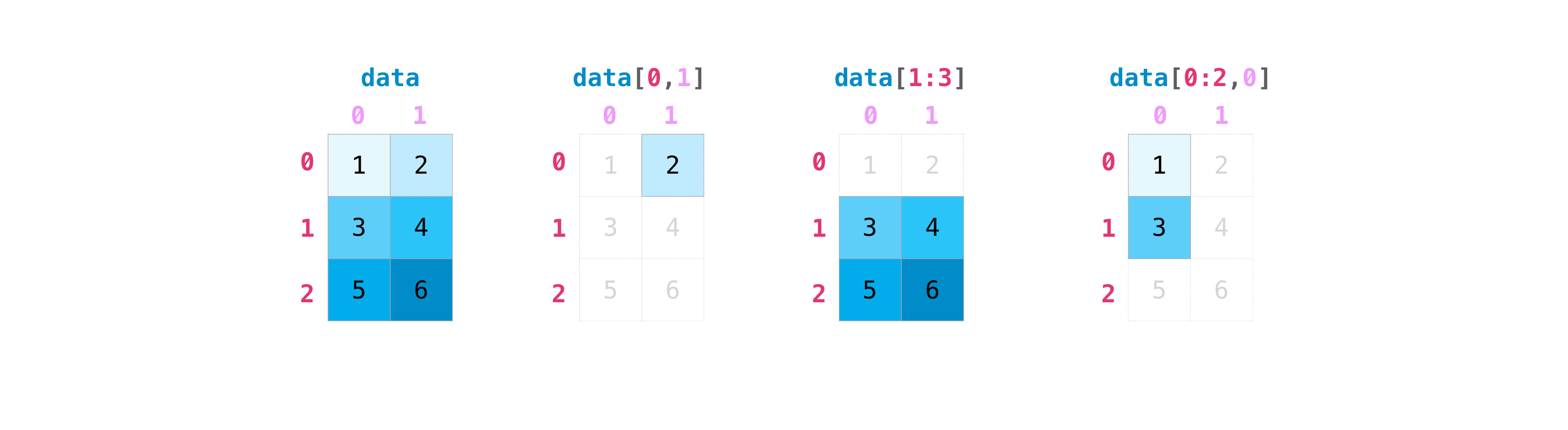
Let’s spend a bit more time on the second indexing example (data[1:3]), which I personally find most confusing because it contains an assumption. First, lets note that the two other indexing operations have a comma between the coordinates, explicitly indicating what to do on each dimension of the array.
data[0:2, 0] can be read as “take rows 0 to 2 (excluded) and column 0”.
data[1:3] in turn can be read as “take rows 1 to 3 (excluded) and all columns”. The “all columns” is implicit (hidden) in the command above, which is why I sometimes prefer the more explicit:
data[1:3, :] # colon means "all elements"
array([[3, 4],
       [5, 6]])
Which does the same but explicitly states “take all columns”.
Q: what do you think will be the output of data[:, :]?
Q: based on the example above and maybe a web search, formulate for yourself what is mean by “slicing” in numpy.
Selecting parts of an array with positional indexing#
Slicing is one way to index parts of a numpy array. It is useful when the area you want to select is structured, e.g. to select only one point or a range of an array as in the example above. Sometimes however you may want to select parts of an array based on other considerations, such as the location of multiple points or based on a condition. Let’s get back to our previous example:
data = np.array([[1, 2], [3, 4], [5, 6]])
data
array([[1, 2],
       [3, 4],
       [5, 6]])
Let’s start with positional indexing (or integer array indexing). Integer array indexing allows selection of arbitrary items in the array based on their N-dimensional index. Each integer array represents a number of indices into that dimension:
data[[0, 2], [1, 1]]
array([2, 6])
In your head, you might want to read this as: “we are extracting elements at locations (0, 1) and (2, 1)”. A bit like putting these two together in an array (but faster):
np.array([data[0, 1], data[2, 1]])
array([2, 6])
This means that if the length of the two integer arrays do not match, numpy will raise an error:
data[[0, 2], [1, 1, 0]] # won't work
---------------------------------------------------------------------------
IndexError                                Traceback (most recent call last)
Cell In[15], line 1
----> 1 data[[0, 2], [1, 1, 0]]  # won't work

IndexError: shape mismatch: indexing arrays could not be broadcast together with shapes (2,) (3,)
Note that it is totally possible so select the same location several times, and also to use negative indexes like for slicing:
data[[0, 0, 2, -1], [1, 1, 1, 0]]
array([2, 2, 6, 5])
Selecting parts of an array with boolean indexing#
Boolean indexing allows to select parts on an array according to a condition of your choice. For example:
data
array([[1, 2],
       [3, 4],
       [5, 6]])
data[data > 2]
array([3, 4, 5, 6])
This is called boolean indexing because what actually matters is the type of data > 2.
np.nonzero and indexing#
np.nonzero is another way to do indexing based on a condition, but with a slightly different workflow and use cases:
indices = np.nonzero(data > 2)
indices
(array([1, 1, 2, 2]), array([0, 1, 0, 1]))
np.nonzero returns a tuple of arrays, one for each dimension of data, containing the indices of the non-zero elements in that dimension. These can then be used for statistics, or as positional indexers:
data[indices[0], indices[1]]
array([3, 4, 5, 6])
Which is the equivalent of data[data > 2]! If you have the choice between the two, boolean indexing (data[data > 2]) is faster and better than using np.nonzero, but sometimes np.nonzero is useful as well (see homework).
Replacing data in ndarrays#
To replace elements in a ndarray, indexing has to be applied on the left-hand side of the assignment operator. For example:
a = np.array([1, 2, 3])
a[1] = 99
a
array([ 1, 99, 3])
If indexing on the left-hand side is more complex (slicing, positional or boolean indexing), the values on the right have to be either scalars, or match the shape of the selection. Here are some examples:
data = np.array([[1, 2], [3, 4], [5, 6]])
data[1:3] = 99
data
array([[ 1,  2],
       [99, 99],
       [99, 99]])
data[1:3] = [[96, 97], [98, 99]]
data
array([[ 1,  2],
       [96, 97],
       [98, 99]])
data[[0, 0], [0, 1]] = 100
data
array([[100, 100],
       [ 96,  97],
       [ 98,  99]])
According to the examples above, and like python lists, ndarrays are mutable objects. This is very important to remember always. For example, the following example should be more or less clear:
a = np.array([1, 2, 3])
b = a
b[1] = 99
a
array([ 1, 99, 3])
Q: is it clear why a was changed as well? If not, ask in class!
Now, with numpy indexing, an additional layer of complexity arises. Some indexing operations (categorized as “basic indexing”) also return what is called a view of an array. See for example:
a = np.array([1, 2, 3])
b = a[1:]
b[0] = 99
a
array([ 1, 99, 3])
Slicing is basic indexing, and it always returns a view. Positional or boolean indexing is “advanced” indexing a returns a copy:
a = np.array([1, 2, 3])
b = a[[1, 2]]
b[0] = 99
a
array([1, 2, 3])
You will have to learn the details of “basic” and “advanced” indexing in more details in the master lecture. For now, remember this pitfall. If you want to make sure to manipulate copies of arrays, you can always make a copy:
a = np.array([1, 2, 3])
b = a[1:].copy()  # make a copy of the sliced array
b[0] = 99
a  # nothing changed in a
array([1, 2, 3])
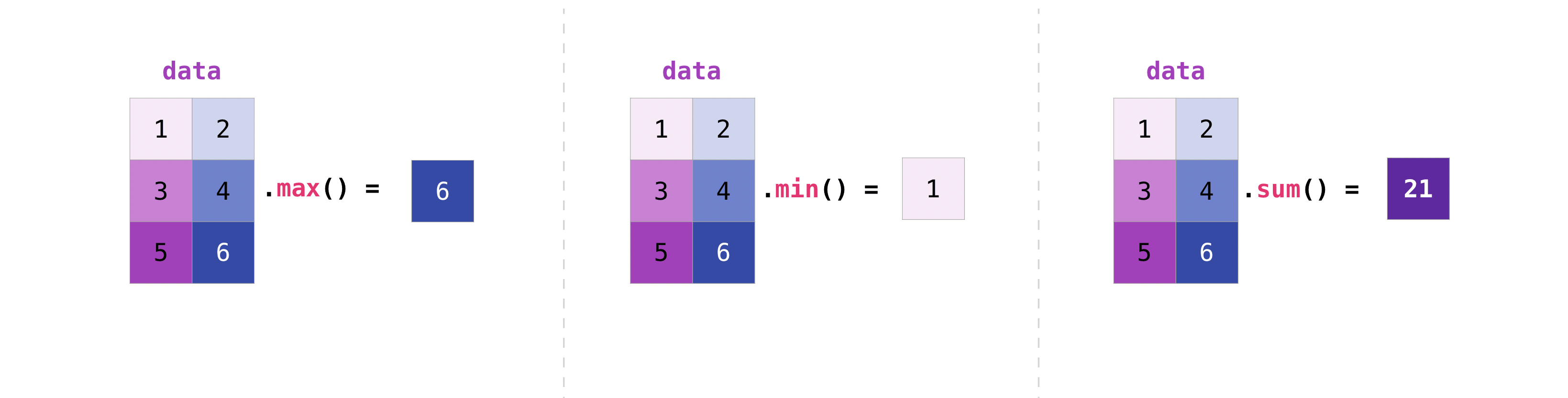
Array statistics (aggregation)#
You can aggregate nD arrays the same way you aggregated 1D arrays:
data = np.array([[1, 2], [3, 4], [5, 6]])
data
array([[1, 2],
       [3, 4],
       [5, 6]])
data.max()
6
data.min()
1
data.sum()
21
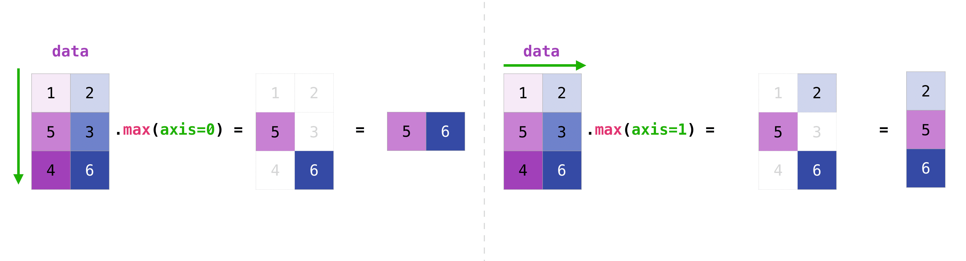
You can aggregate all the values in a matrix and you can aggregate them across columns or rows using the axis parameter. To illustrate this point, let’s look at a slightly modified dataset:
data = np.array([[1, 2], [5, 3], [4, 6]])
data
array([[1, 2],
       [5, 3],
       [4, 6]])
data.max(axis=0)
array([5, 6])
data.max(axis=1)
array([2, 5, 6])
np.meshgrid#
np.meshgrid is a very useful numpy function for grids and gridded data which are so common in physics and geosciences. It allows to create coordinate matrices from coordinate vectors:
x = np.array([1, 2, 3, 4])
y = np.array([-1, 0, 1])
xx, yy = np.meshgrid(x, y)
xx
array([[1, 2, 3, 4],
       [1, 2, 3, 4],
       [1, 2, 3, 4]])
yy
array([[-1, -1, -1, -1],
       [ 0,  0,  0,  0],
       [ 1,  1,  1,  1]])
This is useful to generate 2D fields, but also for plotting, selection by coordinates, and more.
How to save and load NumPy objects#
You will learn about several data formats used commonly in the geosciences next week, and especially next semester in the climate lecture. In the meantime, have a look at this short section in the numpy tutorial. You will need to read .npy files for your homework.
numpy - continued#
I highly recommend to learn the details of numpy at your own pace. The documentation is truly excellent:
The numpy tutorials for beginners to revisit many of the concepts (and learn a few new ones)
The numpy fundamentals are excellent as well. At this stage, I recommend the tutorials “array creation” to “broadcasting”
Plotting 2D arrays#
3D arrays (or more) cannot be plotted on a static flat image easily. 2D data, however, is plotted all the time. Here are a few recipes for you to start with. Plotting with matplotlib offers a very wide range of options and possibilities, sometimes confusing. I can’t teach you all of it now: you will learn the details during the course of your studies and practice!
I recommend to quickly scroll through the following documentation pages, which will give you an overview of matplotlib’s capabilities:
imshow#
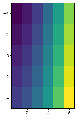
plt.imshow is the simplest way to display an RGB image or assign a color to a value in a 2D array:
x = np.array([1, 2, 3, 4, 5, 6])
y = np.array([-4, -2, 0, 2, 4])
xx, yy = np.meshgrid(x, y)
data = xx**2 + yy
data
array([[-3,  0,  5, 12, 21, 32],
       [-1,  2,  7, 14, 23, 34],
       [ 1,  4,  9, 16, 25, 36],
       [ 3,  6, 11, 18, 27, 38],
       [ 5,  8, 13, 20, 29, 40]])
f, ax = plt.subplots()
im = ax.imshow(data);
f.colorbar(im);
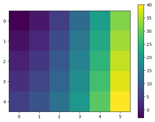
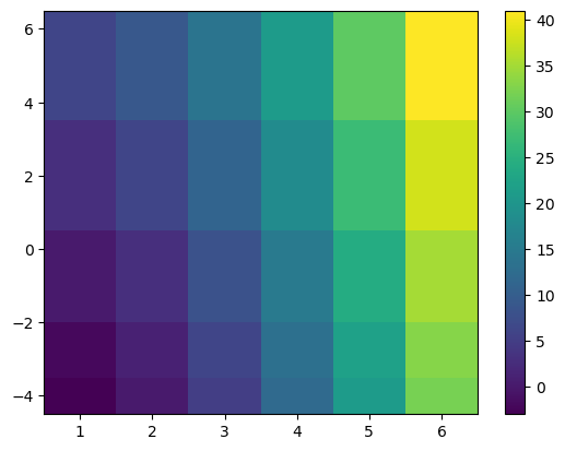
Note the x and y coordinates of the plot. They to not correspond to the one we generated (how could they? imshow was not told about them). If you want the coordinates to show up properly, you will have to indicate them:
plt.imshow(data, extent=(x[0], x[-1], y[-1], y[0]));
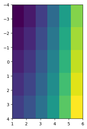
Actually, this is still wrong! The correct way is to indicate the corner coordinates, which is a bit more work and implies to know the spatial resolution of the data:
plt.imshow(data, extent=(x[0]-0.5, x[-1]+0.5, y[-1]+1, y[0]-1));
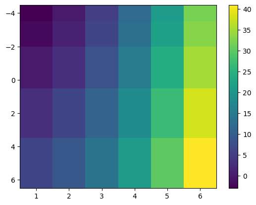
pcolormesh#
pcolormesh is a slower, more flexible solution to the problem of displaying 2D data on screen. Unlike imshow, it allows coordinates as input, and these coordinates do not have to be regularly spaced:
x = np.array([1, 2, 3, 4, 5, 6])
y = np.array([-4, -3, -1, 2, 5])
xx, yy = np.meshgrid(x, y)
data = xx**2 + yy
data
array([[-3,  0,  5, 12, 21, 32],
       [-2,  1,  6, 13, 22, 33],
       [ 0,  3,  8, 15, 24, 35],
       [ 3,  6, 11, 18, 27, 38],
       [ 6,  9, 14, 21, 30, 41]])
f, ax = plt.subplots()
im = ax.pcolormesh(x, y, data, shading='nearest');
f.colorbar(im);
Note that it also takes decisions on the direction of the y-axis based on the data. This is often a good idea, but can be changed of course:
f, ax = plt.subplots()
im = ax.pcolormesh(x, y, data, shading='nearest');
ax.invert_yaxis();
f.colorbar(im);
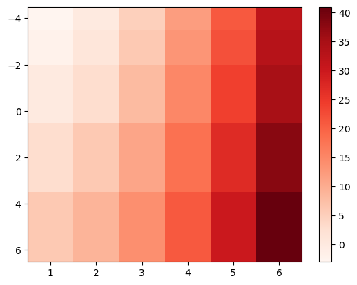
Of course, you can change aspects of the plot such as the colormap to use:
f, ax = plt.subplots()
im = ax.pcolormesh(x, y, data, shading='nearest', cmap='Reds');
ax.invert_yaxis();
f.colorbar(im);
contour and contourf#
Contours are leaving the “pixel space” to make smooth contour fields around the data points.
f, ax = plt.subplots()
cf = ax.contourf(x, y, data, levels=np.arange(0, 40, 2), cmap='inferno', extend='both');
f.colorbar(cf);
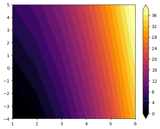
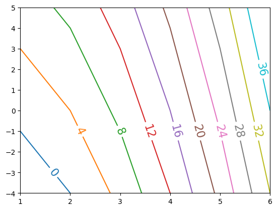
contourf fills with colors, while contour draws lines that can be annotated:
f, ax = plt.subplots()
c = ax.contour(x, y, data, levels=np.arange(0, 40, 4), cmap='tab10', extend='both');
ax.clabel(c, inline=True, fontsize=16);
Learning checklist#