Assignment 06

Due date: 10.05.2023

This week’s assignment has to be returned in the form a jupyter notebook.

Don’t forget the instructions!

01 - Linear regression function

Write a function that computes the parameters \(a\) und \(b\) from the simple linear regression \(\hat{y} = a + bx\), where \(x\) is the explanatory variable and \(y\) the variable to approximate:

\[\begin{split} \begin{eqnarray} b & = & \frac{n\sum_{i=1}^n x_iy_i - \sum_{i=1}^n x_i \sum_{i=1}^ny_i} {n\sum_{i=1}^n (x_i)^2 - (\sum_{i=1}^n x_i)^2} \\ a & = & \overline{y} - b\overline{x} \end{eqnarray} \end{split}\]

In the equation above, \(x_i\) is the i-th element of the vector \(x\), \(n\) is the length (size) of the vectors \(x\) and \(y\), and \(\overline{x}\) is the average of \(x\).

The signature of the function you have to write is given below:

def linear_regression(x, y):
    """Calculate a linear least-squares regression for two sets of measurements.

    Parameters
    ----------
    x, y: ndarray-like
        Two sets of measurements. Both arrays should be 1-dimensional 
        and have the same length. They should not contain any missing data!

    Returns
    -------
    (a, b): floats
       Parameters a and b of the linear approximation y^ = a + b x

    Examples
    --------
    >>> x = np.array([1, 2, 3, 4, 5])
    >>> y = np.array([-5.3, -2.6,  0.1,  2.8,  5.5])
    >>> a, b = linear_regression(x, y)
    >>> np.isclose(a, -8)
    True
    >>> np.isclose(b, 2.7)
    True
    """
    # Make sure we manipulate ndarrays
    x = np.asarray(x)
    y = np.asarray(y)

    # Least squares equations
    < your code here >
    return a, b

# Your answer here

If you have written the function correctly, the tests should pass with TestResults(failed=0, attempted=5):

# Testing
import doctest
doctest.testmod()

TestResults(failed=0, attempted=0)

02 - Instrument calibration

A temperature sensor was calibrated in a precise temperature chamber. The instrument provides an analog output signal of varying voltage in Volts (V) on a single pin that can be measured. The temperature in the chamber T is increased from -20°C to 40°C in 2°C increments, and the sensor voltage is measured after the temperature in the chamber is stabilized.

The data is stored in a comma-separated file calibration.csv. Download the data file (right click + “Save as…”) and put the file in the same folder as this notebook. Explore the csv file by opening it in JupyterLab.

A few weeks ago, you wrote your own text file reader. This time, let me read the data for you using numpy:

import numpy as np
t, v = np.genfromtxt('calibration.csv', delimiter=',', skip_header=1, unpack=True)

Something happened during the experiment, and unfortunately some of the values are invalid with the missing value indicator -999. Filter the data series so that both t and v are of the same length and still represent the correct value pairs, without missing data.

# Your answer here

Plot the voltage values v as a function of the temparature chamber t on a scatter plot. Label the x and y axis accordingly.

# Your answer here

Using your linear regression function, find the sensor calibration parameters a and b, so that the temperature t can be reconstructed from the voltage measurements with \(\hat{t} = a + b v\).

# Your answer here

The sensor and associated voltmeter are designed to output a voltage going from 0V to 12V. Based on your calibration values, what is the sensor’s valid temperature range?

# Your answer here

Compute the reconstructed temperature tr (volts converted to temperature).

# Your answer here

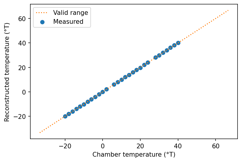
Plot the chamber temperature, the reconstructed temperature (volts converted to temperature) and the valid range in one plot. The plot should look somewhat similar to this example.

# Your answer here

Compute the accuracy of the sensor assuming that the chamber temperature is truly exact. To evaluate the accuracy, compute the root mean square deviation as:

\[ RMSD = \sqrt{\overline{(\hat{t} - t)^2}} \]

Where \(\hat{t}\) is the reconstructed temperature, and the overline represents the average (mean) of the squared deviation \((\hat{t} - t)^2\).

# Your answer here